Methodology, Parameters, and Calculations
Keywords
health economics methodology, clinical trial cost analysis, medical research ROI, cost-benefit analysis healthcare, sensitivity analysis, Monte Carlo simulation, DALY calculation, pragmatic clinical trials
Overview
This appendix documents all 238 parameters used in the analysis, organized by type:
- External sources (peer-reviewed): 94
- Calculated values: 111
- Core definitions: 33
Calculated Values
Parameters derived from mathematical formulas and economic models.
Additional Drug Approvals from Cost Elimination: 20 drugs/year
Note📊 Details
Additional drug approvals per year when Phase 2/3 cost barrier eliminated. Assumes valley-of-death compounds (abandoned due to cost) would have similar success rate to funded compounds.
Inputs:
- Average Annual New Drug Approvals Globally 📊: 50 drugs/year (95% CI: 45 drugs/year - 60 drugs/year)
- Valley of Death Attrition Rate 📊: 40% (95% CI: 25% - 55%)
\[ \begin{gathered} Drugs_{new} \\ = Drugs_{ann,curr} \times Attrition_{valley} \\ = 50 \times 40\% \\ = 20 \end{gathered} \]
~ Medium confidence
Sensitivity Analysis
Sensitivity Indices for Additional Drug Approvals from Cost Elimination
Regression-based sensitivity showing which inputs explain the most variance in the output.
| Input Parameter | Sensitivity Coefficient | Interpretation |
|---|---|---|
| Average Annual New Drug Approvals Globally (drugs/year) | 1.0000 | Strong driver |
Interpretation: Standardized coefficients show the change in output (in SD units) per 1 SD change in input. Values near ±1 indicate strong influence; values exceeding ±1 may occur with correlated inputs.
Monte Carlo Distribution
Simulation Results Summary: Additional Drug Approvals from Cost Elimination
| Statistic | Value |
|---|---|
| Baseline (deterministic) | 20 |
| Mean (expected value) | 20 |
| Median (50th percentile) | 19.9 |
| Standard Deviation | 1.42 |
| 90% Range (5th-95th percentile) | [18, 22.6] |
The histogram shows the distribution of Additional Drug Approvals from Cost Elimination across 10,000 Monte Carlo simulations. The CDF (right) shows the probability of the outcome exceeding any given value, which is useful for risk assessment.
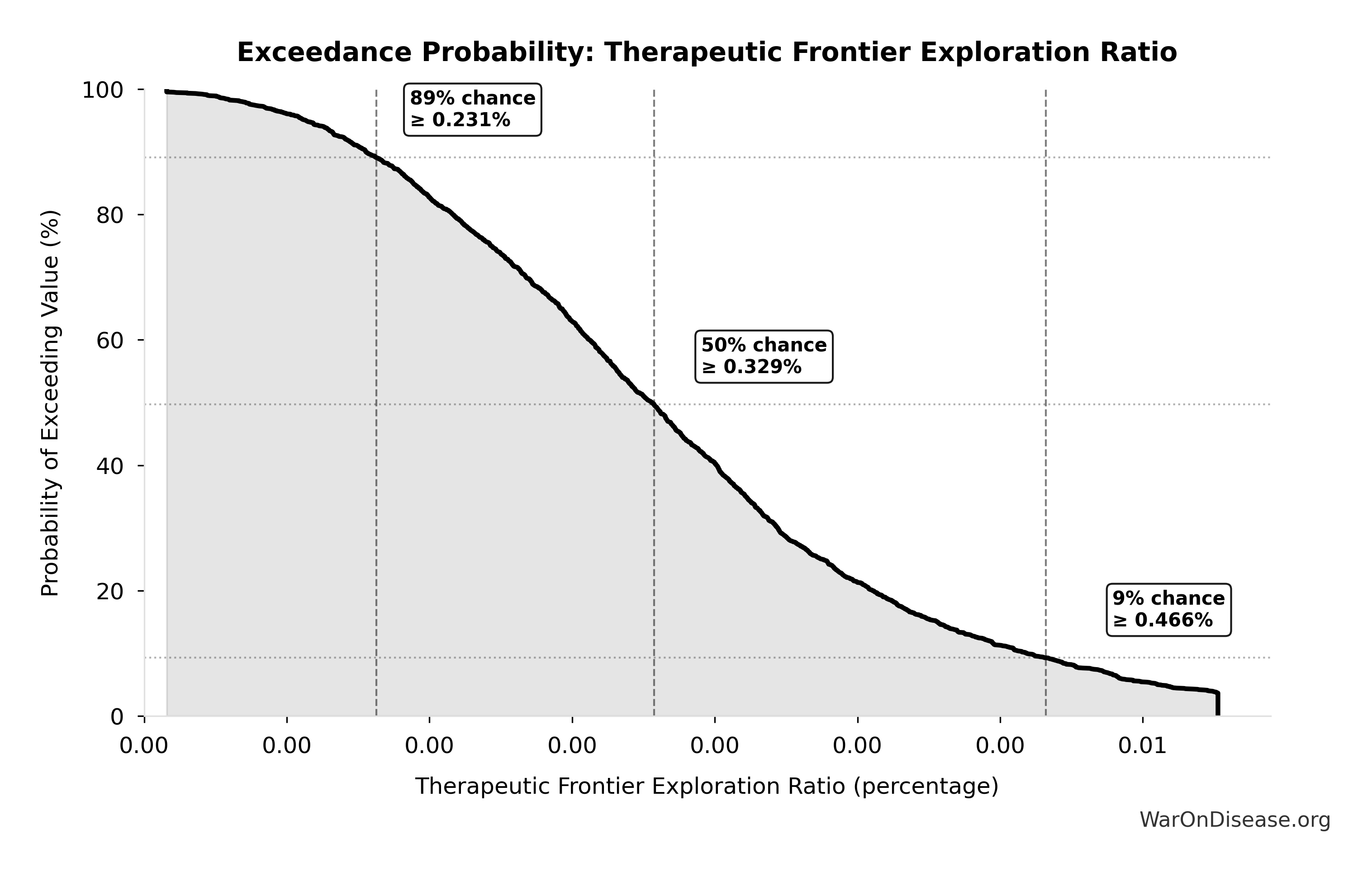
Exceedance Probability
This exceedance probability chart shows the likelihood that Additional Drug Approvals from Cost Elimination will exceed any given threshold. Higher curves indicate more favorable outcomes with greater certainty.
Combination Therapy Space: 45.1 billion combinations
Note📊 Details
Total combination therapy space (pairwise drug combinations × diseases). Standard in oncology, HIV, cardiology.
Inputs:
- Pairwise Drug Combinations 🔢: 45.1 million combinations
- Trial-Relevant Diseases: 1 thousand diseases (95% CI: 800 diseases - 1.2 thousand diseases)
\[ \begin{gathered} Space_{combo} \\ = N_{combo} \times N_{diseases,trial} \\ = 45.1M \times 1{,}000 \\ = 45.1B \end{gathered} \]
✓ High confidence
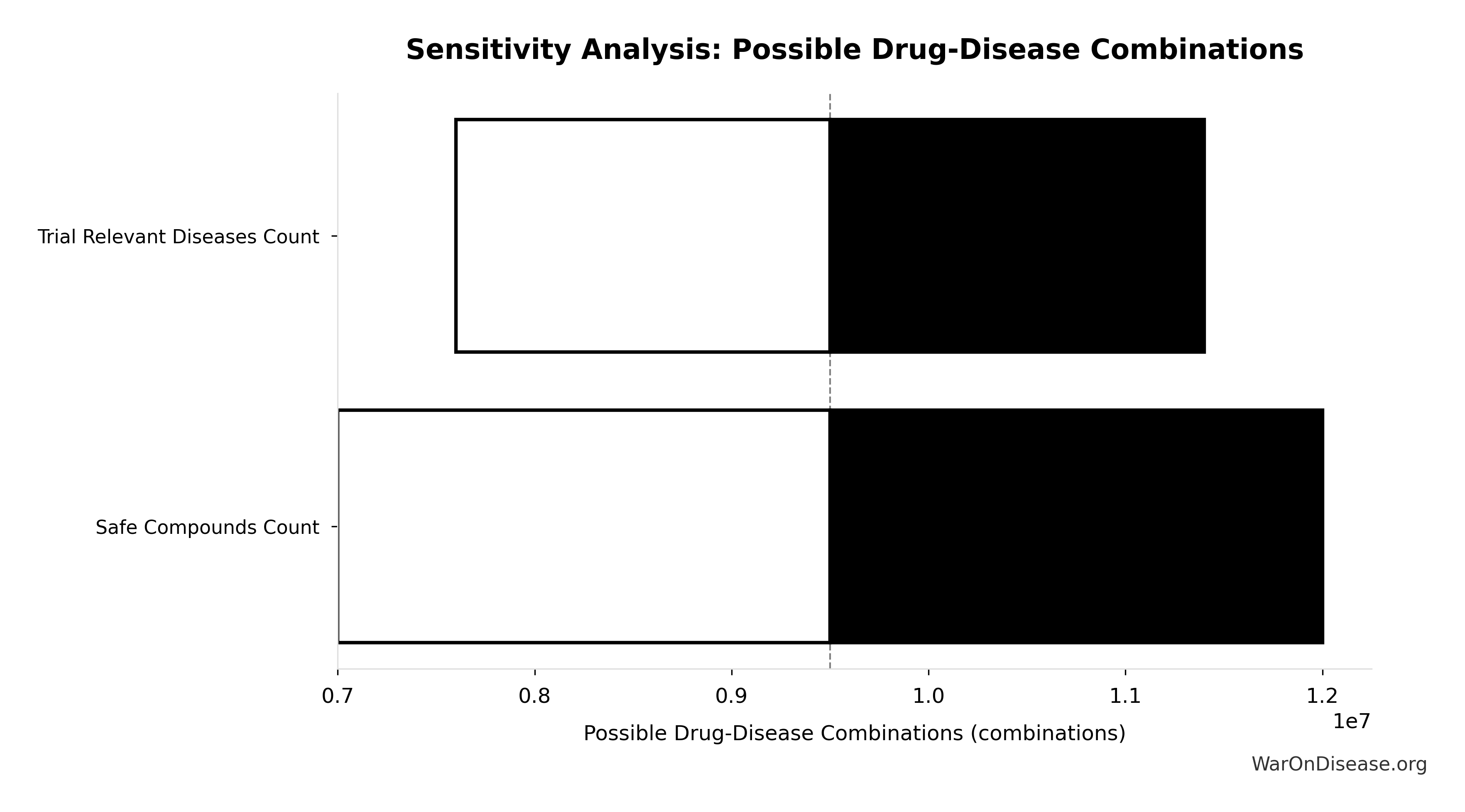
Sensitivity Analysis
Pairwise Drug Combinations: 45.1 million combinations
Note📊 Details
Unique pairwise drug combinations from known safe compounds (n choose 2)
Inputs:
- Safe Compounds Available for Testing: 9.5 thousand compounds (95% CI: 7 thousand compounds - 12 thousand compounds)
Formula: SAFE_COMPOUNDS × (SAFE_COMPOUNDS - 1) ÷ 2
✓ High confidence
Sensitivity Analysis
Combination Therapy Exploration Time (Current): 13.7 million years
Note📊 Details
Years to test all pairwise drug combinations at current trial capacity. Combination therapy is standard in oncology, HIV, cardiology.
Inputs:
- Combination Therapy Space 🔢: 45.1 billion combinations
- Current Global Clinical Trials per Year 📊: 3.3 thousand trials/year (95% CI: 2.64 thousand trials/year - 3.96 thousand trials/year)
\[ \begin{gathered} T_{explore,combo} \\ = \frac{Space_{combo}}{Trials_{ann,curr}} \\ = \frac{45.1B}{3{,}300} \\ = 13.7M \end{gathered} \] where: \[ \begin{gathered} Space_{combo} \\ = N_{combo} \times N_{diseases,trial} \\ = 45.1M \times 1{,}000 \\ = 45.1B \end{gathered} \] ✓ High confidence
Sensitivity Analysis
Sensitivity Indices for Combination Therapy Exploration Time (Current)
Regression-based sensitivity showing which inputs explain the most variance in the output.
| Input Parameter | Sensitivity Coefficient | Interpretation |
|---|---|---|
| Current Global Clinical Trials per Year (trials/year) | -0.9931 | Strong driver |
Interpretation: Standardized coefficients show the change in output (in SD units) per 1 SD change in input. Values near ±1 indicate strong influence; values exceeding ±1 may occur with correlated inputs.
Monte Carlo Distribution

Simulation Results Summary: Combination Therapy Exploration Time (Current)
| Statistic | Value |
|---|---|
| Baseline (deterministic) | 13.7 million |
| Mean (expected value) | 13.8 million |
| Median (50th percentile) | 13.8 million |
| Standard Deviation | 1.36 million |
| 90% Range (5th-95th percentile) | [11.6 million, 16.3 million] |
The histogram shows the distribution of Combination Therapy Exploration Time (Current) across 10,000 Monte Carlo simulations. The CDF (right) shows the probability of the outcome exceeding any given value, which is useful for risk assessment.
Exceedance Probability

This exceedance probability chart shows the likelihood that Combination Therapy Exploration Time (Current) will exceed any given threshold. Higher curves indicate more favorable outcomes with greater certainty.
Known Safe Exploration Time (Current): 2.88 thousand years
Note📊 Details
Years to test all known safe drug-disease combinations at current global trial capacity
Inputs:
- Possible Drug-Disease Combinations 🔢: 9.5 million combinations
- Current Global Clinical Trials per Year 📊: 3.3 thousand trials/year (95% CI: 2.64 thousand trials/year - 3.96 thousand trials/year)
\[ \begin{gathered} T_{explore,safe} \\ = \frac{N_{combos}}{Trials_{ann,curr}} \\ = \frac{9.5M}{3{,}300} \\ = 2{,}880 \end{gathered} \] where: \[ \begin{gathered} N_{combos} \\ = N_{safe} \times N_{diseases,trial} \\ = 9{,}500 \times 1{,}000 \\ = 9.5M \end{gathered} \] ✓ High confidence
Sensitivity Analysis

Sensitivity Indices for Known Safe Exploration Time (Current)
Regression-based sensitivity showing which inputs explain the most variance in the output.
| Input Parameter | Sensitivity Coefficient | Interpretation |
|---|---|---|
| Current Global Clinical Trials per Year (trials/year) | -0.9931 | Strong driver |
Interpretation: Standardized coefficients show the change in output (in SD units) per 1 SD change in input. Values near ±1 indicate strong influence; values exceeding ±1 may occur with correlated inputs.
Monte Carlo Distribution
Simulation Results Summary: Known Safe Exploration Time (Current)
| Statistic | Value |
|---|---|
| Baseline (deterministic) | 2.88 thousand |
| Mean (expected value) | 2.91 thousand |
| Median (50th percentile) | 2.9 thousand |
| Standard Deviation | 286 |
| 90% Range (5th-95th percentile) | [2.45 thousand, 3.43 thousand] |
The histogram shows the distribution of Known Safe Exploration Time (Current) across 10,000 Monte Carlo simulations. The CDF (right) shows the probability of the outcome exceeding any given value, which is useful for risk assessment.
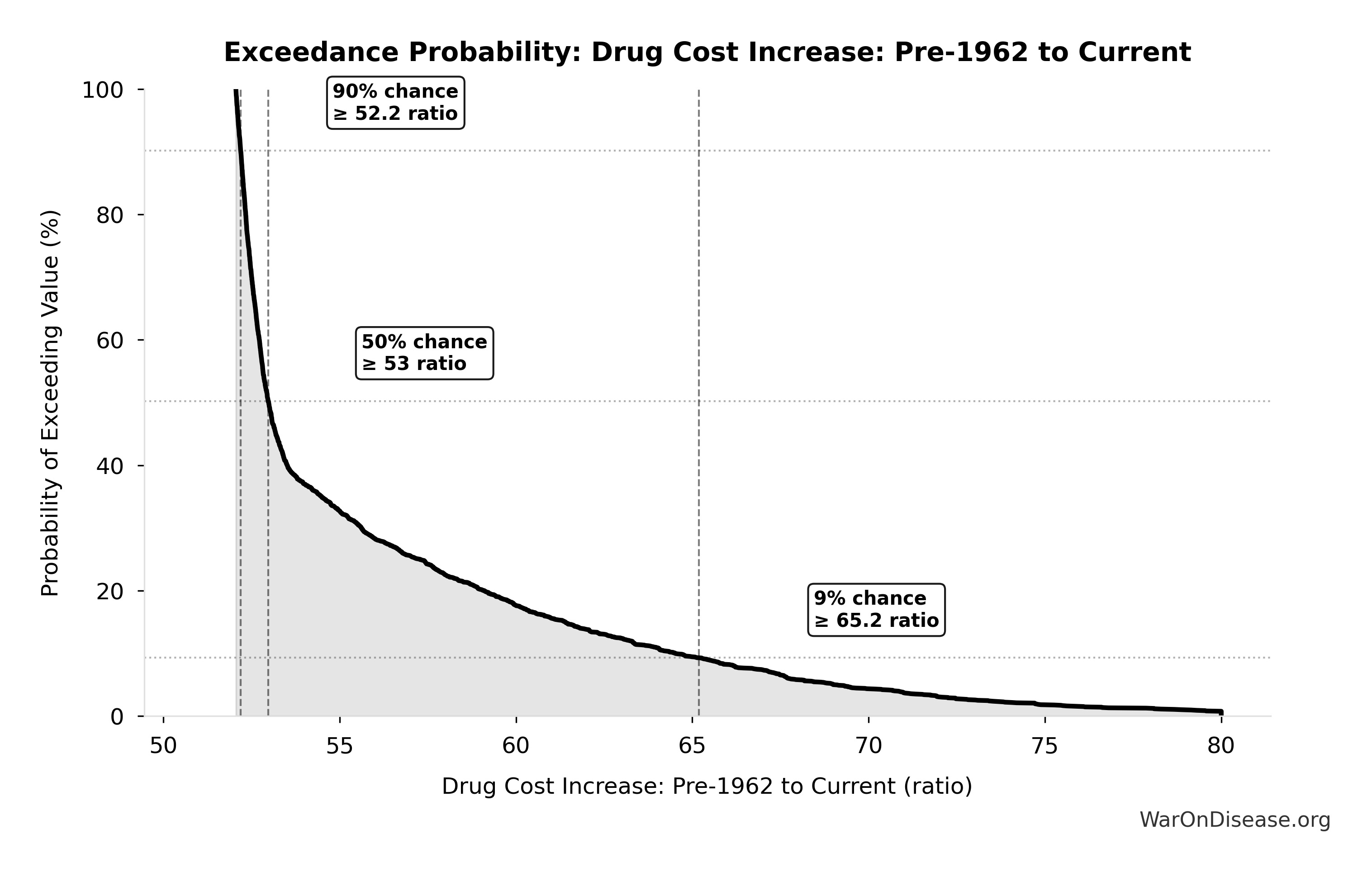
Exceedance Probability
This exceedance probability chart shows the likelihood that Known Safe Exploration Time (Current) will exceed any given threshold. Higher curves indicate more favorable outcomes with greater certainty.
Current Patient Participation Rate in Clinical Trials: 0.0792%
Note📊 Details
Current patient participation rate in clinical trials (0.08% = 1.9M participants / 2.4B disease patients)
Inputs:
- Annual Global Clinical Trial Participants 📊: 1.9 million patients/year (95% CI: 1.5 million patients/year - 2.3 million patients/year)
- Global Population with Chronic Diseases 📊: 2.4 billion people (95% CI: 2 billion people - 2.8 billion people)
\[ \begin{gathered} Rate_{part} \\ = \frac{Slots_{curr}}{N_{patients}} \\ = \frac{1.9M}{2.4B} \\ = 0.0792\% \end{gathered} \]
Methodology:13
✓ High confidence
Sensitivity Analysis
Sensitivity Indices for Current Patient Participation Rate in Clinical Trials
Regression-based sensitivity showing which inputs explain the most variance in the output.
| Input Parameter | Sensitivity Coefficient | Interpretation |
|---|---|---|
| Global Population with Chronic Diseases (people) | 4.1698 | Strong driver |
| Annual Global Clinical Trial Participants (patients/year) | -3.1720 | Strong driver |
Interpretation: Standardized coefficients show the change in output (in SD units) per 1 SD change in input. Values near ±1 indicate strong influence; values exceeding ±1 may occur with correlated inputs.
Monte Carlo Distribution
Simulation Results Summary: Current Patient Participation Rate in Clinical Trials
| Statistic | Value |
|---|---|
| Baseline (deterministic) | 0.0792% |
| Mean (expected value) | 0.079% |
| Median (50th percentile) | 0.079% |
| Standard Deviation | 0.00169% |
| 90% Range (5th-95th percentile) | [0.0761%, 0.0819%] |
The histogram shows the distribution of Current Patient Participation Rate in Clinical Trials across 10,000 Monte Carlo simulations. The CDF (right) shows the probability of the outcome exceeding any given value, which is useful for risk assessment.
Exceedance Probability

This exceedance probability chart shows the likelihood that Current Patient Participation Rate in Clinical Trials will exceed any given threshold. Higher curves indicate more favorable outcomes with greater certainty.
Current Trajectory Average Income at Year 20: $20.5K
Note📊 Details
Average income (GDP per capita) at year 20 under current trajectory trajectory.
Inputs:
- Current Trajectory GDP at Year 20 🔢: $188T
- Global Population 2045 (Projected) 📊: 9.2 billion of people
\[ \begin{gathered} \bar{y}_{base,20} \\ = \frac{GDP_{base,20}}{Pop_{2045}} \\ = \frac{\$188T}{9.2B} \\ = \$20.5K \end{gathered} \] where: \[ GDP_{base,20} = GDP_0(1+g_{base})^{20} \] ✓ High confidence
Monte Carlo Distribution
Simulation Results Summary: Current Trajectory Average Income at Year 20
| Statistic | Value |
|---|---|
| Baseline (deterministic) | $20.5K |
| Mean (expected value) | $20.5K |
| Median (50th percentile) | $20.5K |
| Standard Deviation | $3.64e-12 |
| 90% Range (5th-95th percentile) | [$20.5K, $20.5K] |
The histogram shows the distribution of Current Trajectory Average Income at Year 20 across 10,000 Monte Carlo simulations. The CDF (right) shows the probability of the outcome exceeding any given value, which is useful for risk assessment.
Exceedance Probability
This exceedance probability chart shows the likelihood that Current Trajectory Average Income at Year 20 will exceed any given threshold. Higher curves indicate more favorable outcomes with greater certainty.
Current Trajectory GDP at Year 20: $188T
Note📊 Details
Global GDP at year 20 under status-quo current trajectory growth.
Inputs:
- Global GDP (2025) 📊: $115T
- Baseline Global GDP Growth Rate: 2.5%
\[ GDP_{base,20} = GDP_0(1+g_{base})^{20} \]
✓ High confidence
Monte Carlo Distribution
Simulation Results Summary: Current Trajectory GDP at Year 20
| Statistic | Value |
|---|---|
| Baseline (deterministic) | $188T |
| Mean (expected value) | $188T |
| Median (50th percentile) | $188T |
| Standard Deviation | $0.031 |
| 90% Range (5th-95th percentile) | [$188T, $188T] |
The histogram shows the distribution of Current Trajectory GDP at Year 20 across 10,000 Monte Carlo simulations. The CDF (right) shows the probability of the outcome exceeding any given value, which is useful for risk assessment.
Exceedance Probability
This exceedance probability chart shows the likelihood that Current Trajectory GDP at Year 20 will exceed any given threshold. Higher curves indicate more favorable outcomes with greater certainty.
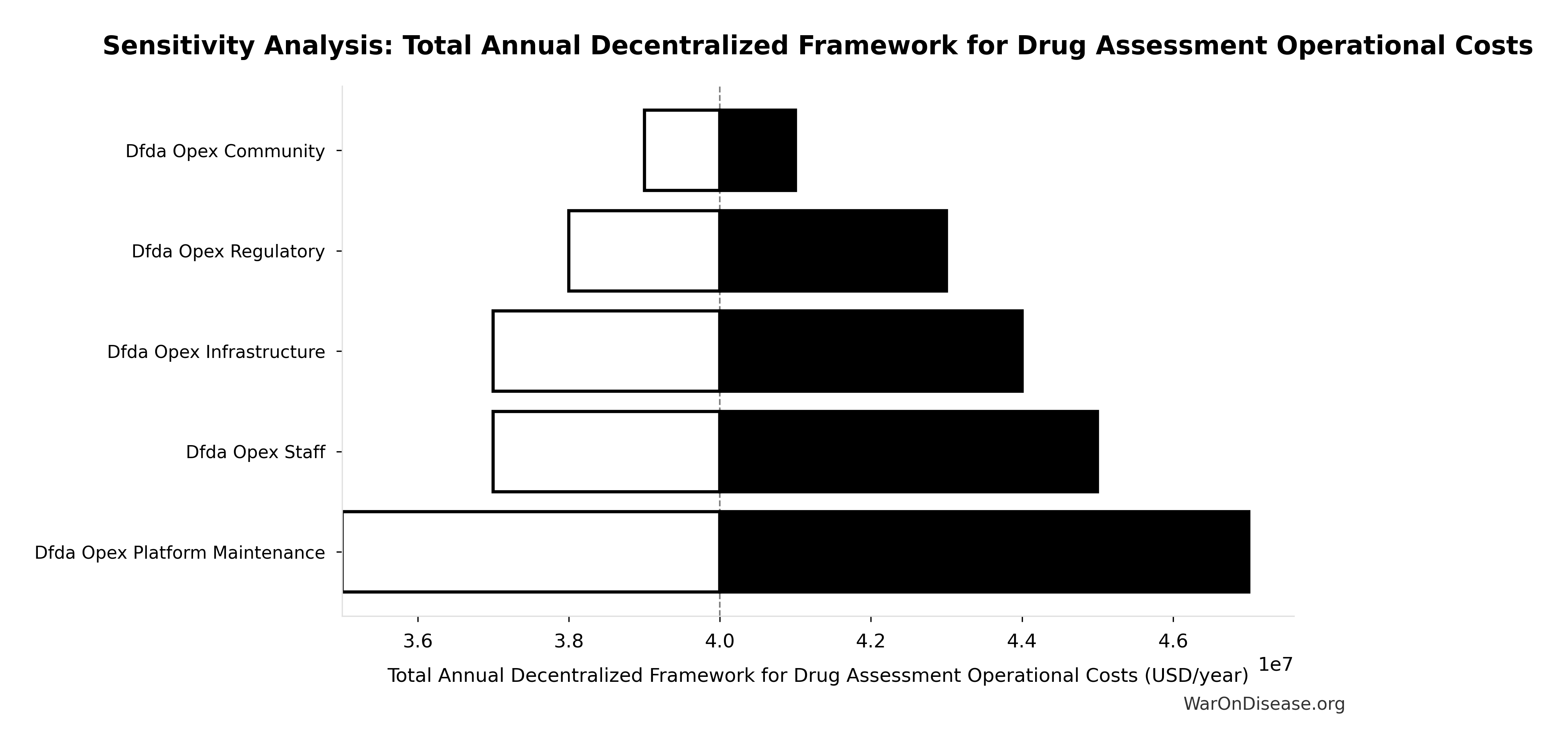
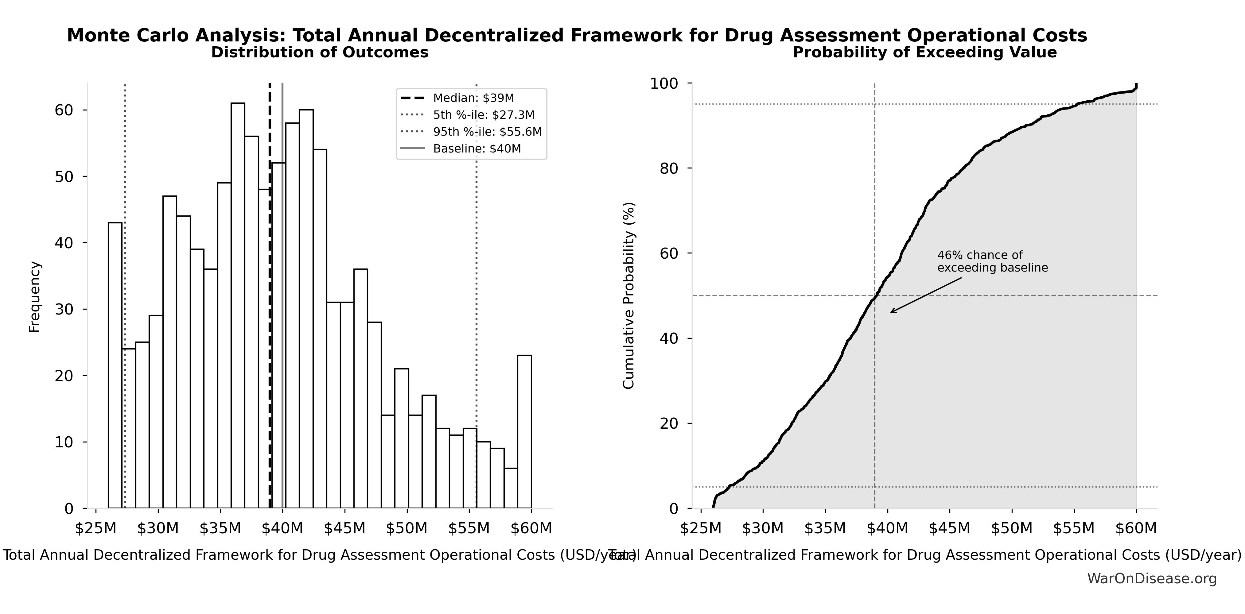
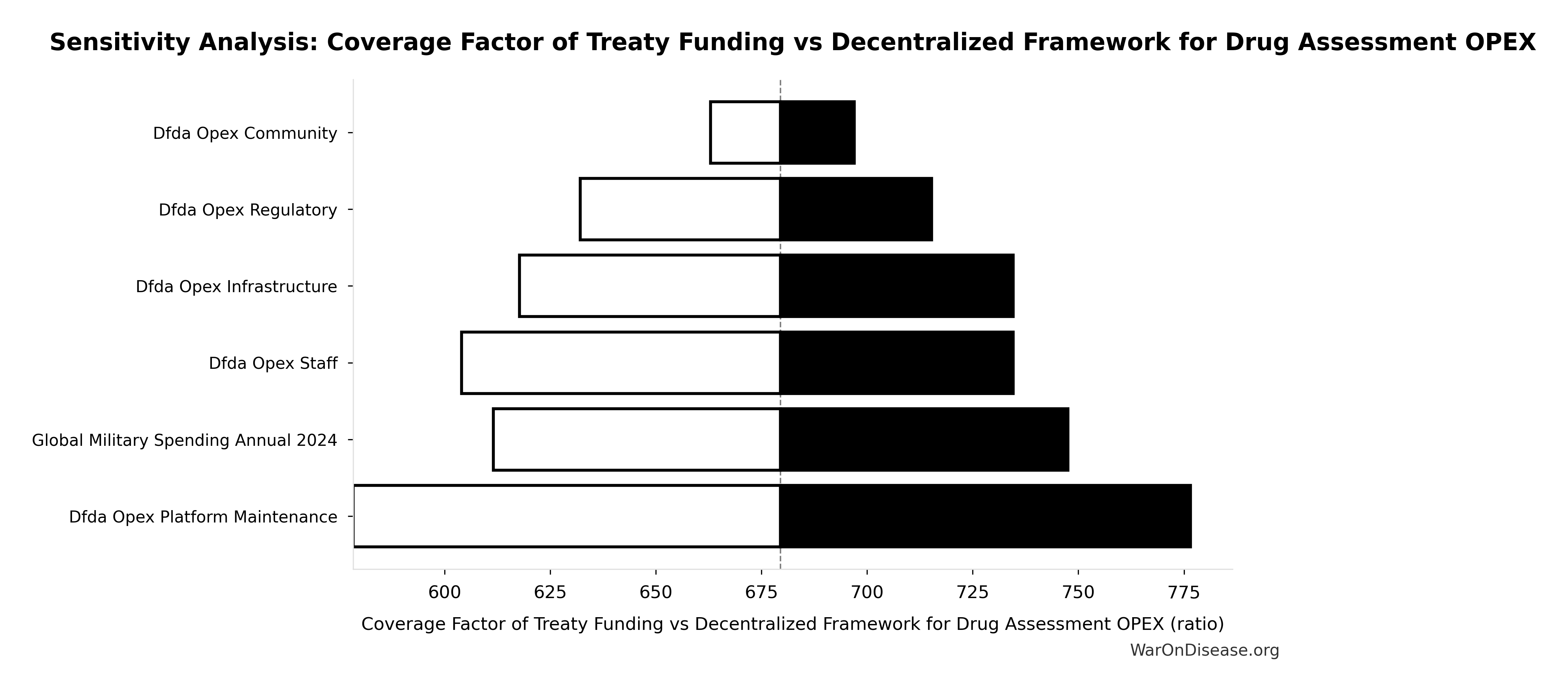
Total Annual Decentralized Framework for Drug Assessment Operational Costs: $40M
Note📊 Details
Total annual Decentralized Framework for Drug Assessment operational costs (sum of all components: platform + staff + infra + regulatory + community)
Inputs:
- Decentralized Framework for Drug Assessment Maintenance Costs: $15M (95% CI: $10M - $22M)
- Decentralized Framework for Drug Assessment Staff Costs: $10M (95% CI: $7M - $15M)
- Decentralized Framework for Drug Assessment Infrastructure Costs: $8M (95% CI: $5M - $12M)
- Decentralized Framework for Drug Assessment Regulatory Coordination Costs: $5M (95% CI: $3M - $8M)
- Decentralized Framework for Drug Assessment Community Support Costs: $2M (95% CI: $1M - $3M)
\[ \begin{gathered} OPEX_{dFDA} \\ = Cost_{platform} + Cost_{staff} + Cost_{infra} \\ + Cost_{regulatory} + Cost_{community} \\ = \$15M + \$10M + \$8M + \$5M + \$2M \\ = \$40M \end{gathered} \]
✓ High confidence
Sensitivity Analysis
Sensitivity Indices for Total Annual Decentralized Framework for Drug Assessment Operational Costs
Regression-based sensitivity showing which inputs explain the most variance in the output.
| Input Parameter | Sensitivity Coefficient | Interpretation |
|---|---|---|
| Decentralized Framework for Drug Assessment Maintenance Costs (USD/year) | 0.3542 | Moderate driver |
| Decentralized Framework for Drug Assessment Staff Costs (USD/year) | 0.2355 | Weak driver |
| Decentralized Framework for Drug Assessment Infrastructure Costs (USD/year) | 0.2060 | Weak driver |
| Decentralized Framework for Drug Assessment Regulatory Coordination Costs (USD/year) | 0.1469 | Weak driver |
| Decentralized Framework for Drug Assessment Community Support Costs (USD/year) | 0.0576 | Minimal effect |
Interpretation: Standardized coefficients show the change in output (in SD units) per 1 SD change in input. Values near ±1 indicate strong influence; values exceeding ±1 may occur with correlated inputs.
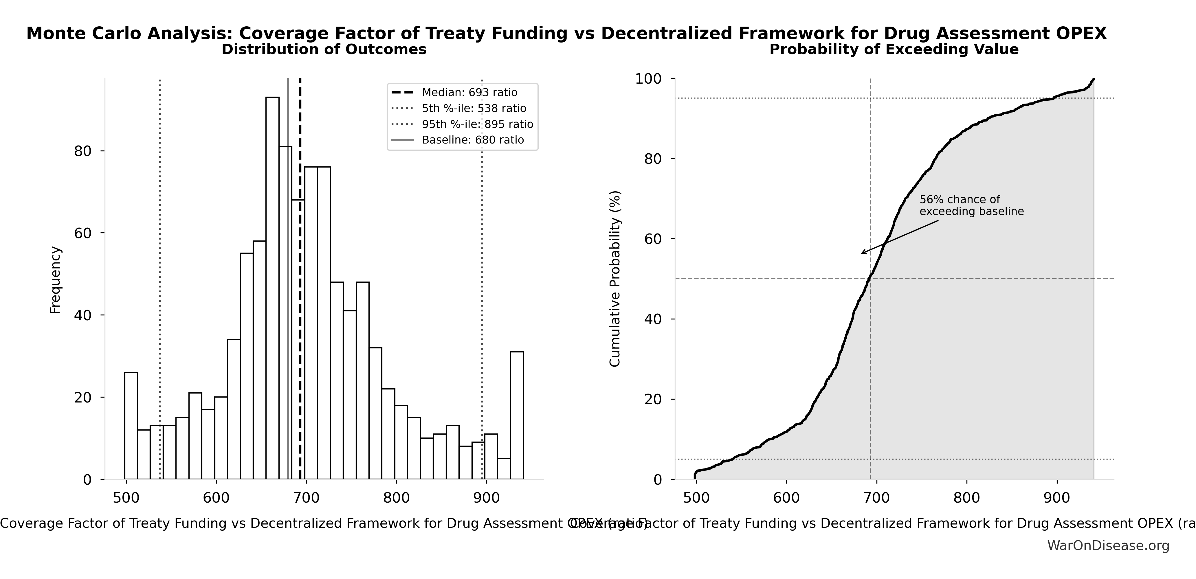
Monte Carlo Distribution
Simulation Results Summary: Total Annual Decentralized Framework for Drug Assessment Operational Costs
| Statistic | Value |
|---|---|
| Baseline (deterministic) | $40M |
| Mean (expected value) | $39.9M |
| Median (50th percentile) | $39M |
| Standard Deviation | $8.21M |
| 90% Range (5th-95th percentile) | [$27.3M, $55.6M] |
The histogram shows the distribution of Total Annual Decentralized Framework for Drug Assessment Operational Costs across 10,000 Monte Carlo simulations. The CDF (right) shows the probability of the outcome exceeding any given value, which is useful for risk assessment.
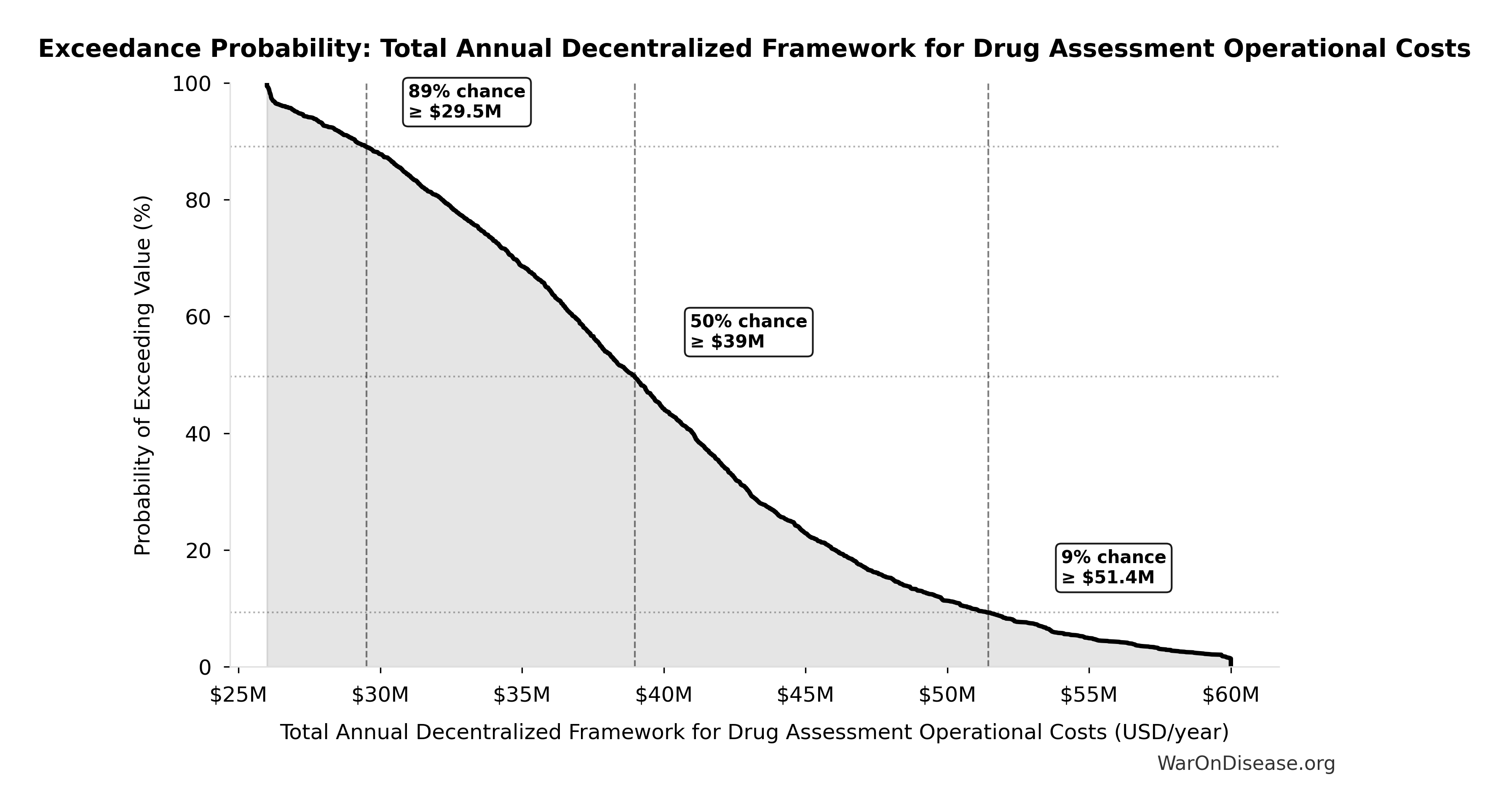
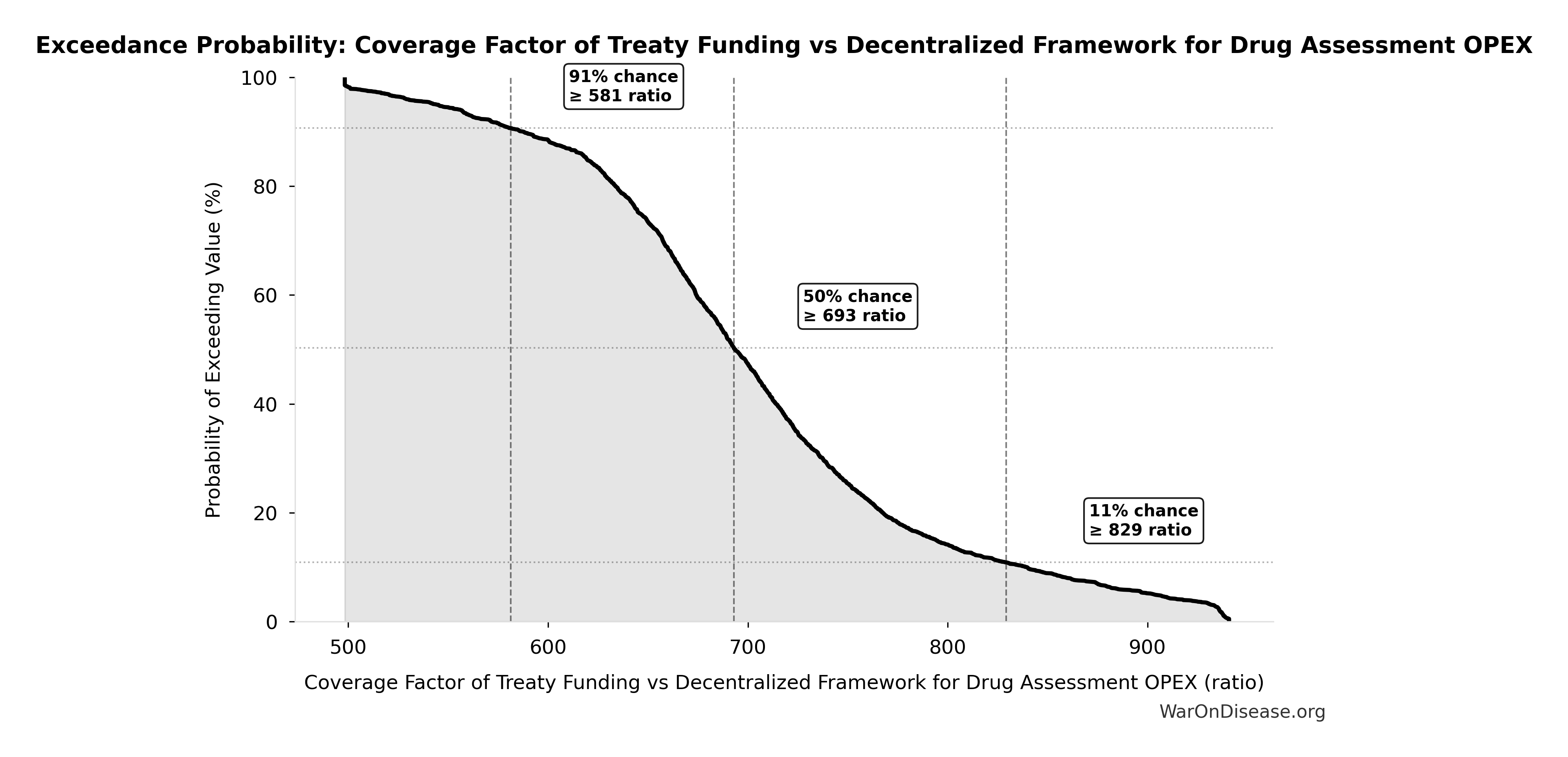
Exceedance Probability
This exceedance probability chart shows the likelihood that Total Annual Decentralized Framework for Drug Assessment Operational Costs will exceed any given threshold. Higher curves indicate more favorable outcomes with greater certainty.
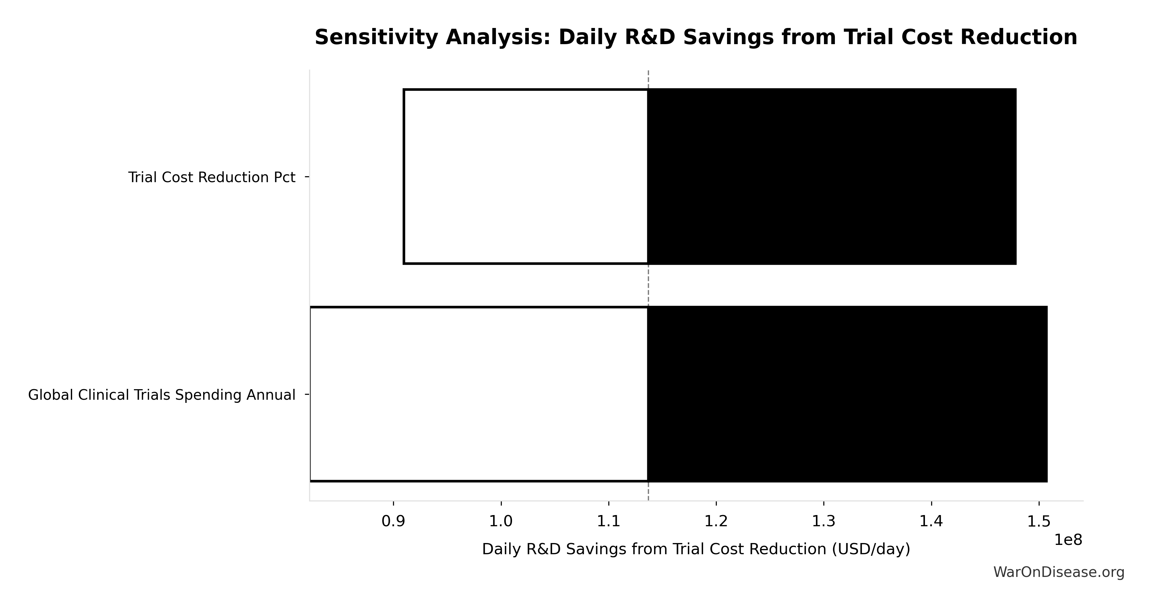
Decentralized Framework for Drug Assessment Annual Benefit: R&D Savings: $58.6B
Note📊 Details
Annual Decentralized Framework for Drug Assessment benefit from R&D savings (trial cost reduction, secondary component)
Inputs:
- Annual Global Spending on Clinical Trials 📊: $60B (95% CI: $50B - $75B)
- dFDA Trial Cost Reduction Percentage 🔢: 97.7%
\[ \begin{gathered} Benefit_{RD,ann} \\ = Spending_{trials} \times Reduce_{pct} \\ = \$60B \times 97.7\% \\ = \$58.6B \end{gathered} \] where: \[ \begin{gathered} Reduce_{pct} \\ = 1 - \frac{Cost_{pragmatic,pt}}{Cost_{P3,pt}} \\ = 1 - \frac{\$929}{\$41K} \\ = 97.7\% \end{gathered} \] ✓ High confidence
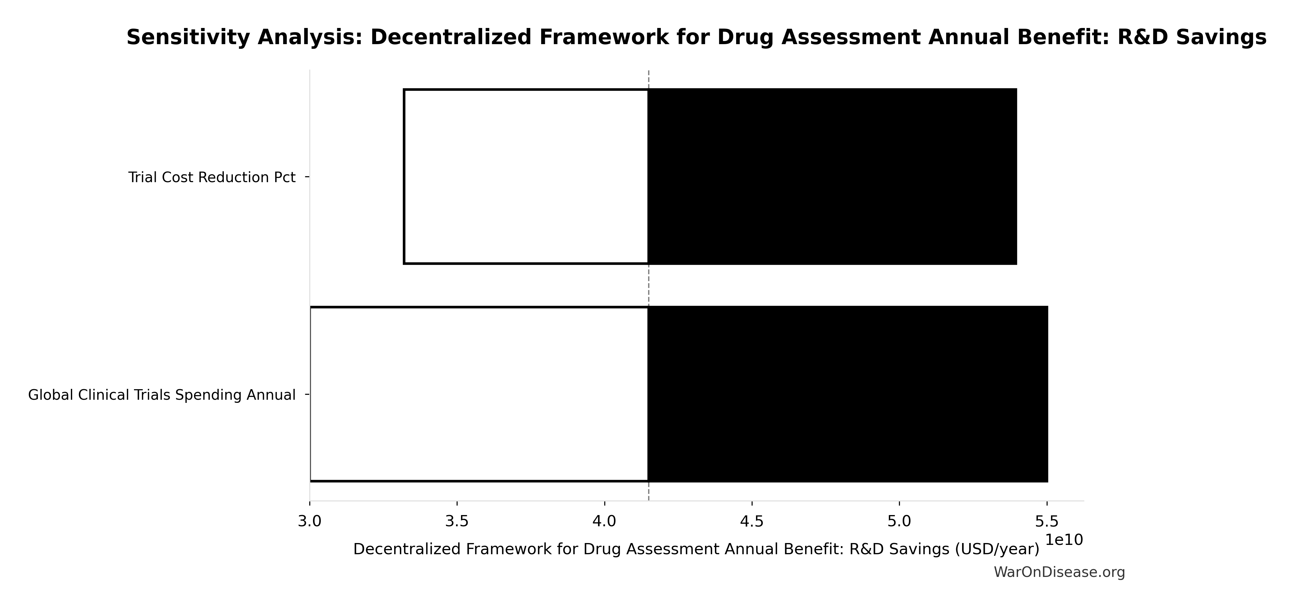
Sensitivity Analysis
Sensitivity Indices for Decentralized Framework for Drug Assessment Annual Benefit: R&D Savings
Regression-based sensitivity showing which inputs explain the most variance in the output.
| Input Parameter | Sensitivity Coefficient | Interpretation |
|---|---|---|
| Annual Global Spending on Clinical Trials (USD) | 1.0205 | Strong driver |
| dFDA Trial Cost Reduction Percentage (percentage) | 0.0244 | Minimal effect |
Interpretation: Standardized coefficients show the change in output (in SD units) per 1 SD change in input. Values near ±1 indicate strong influence; values exceeding ±1 may occur with correlated inputs.
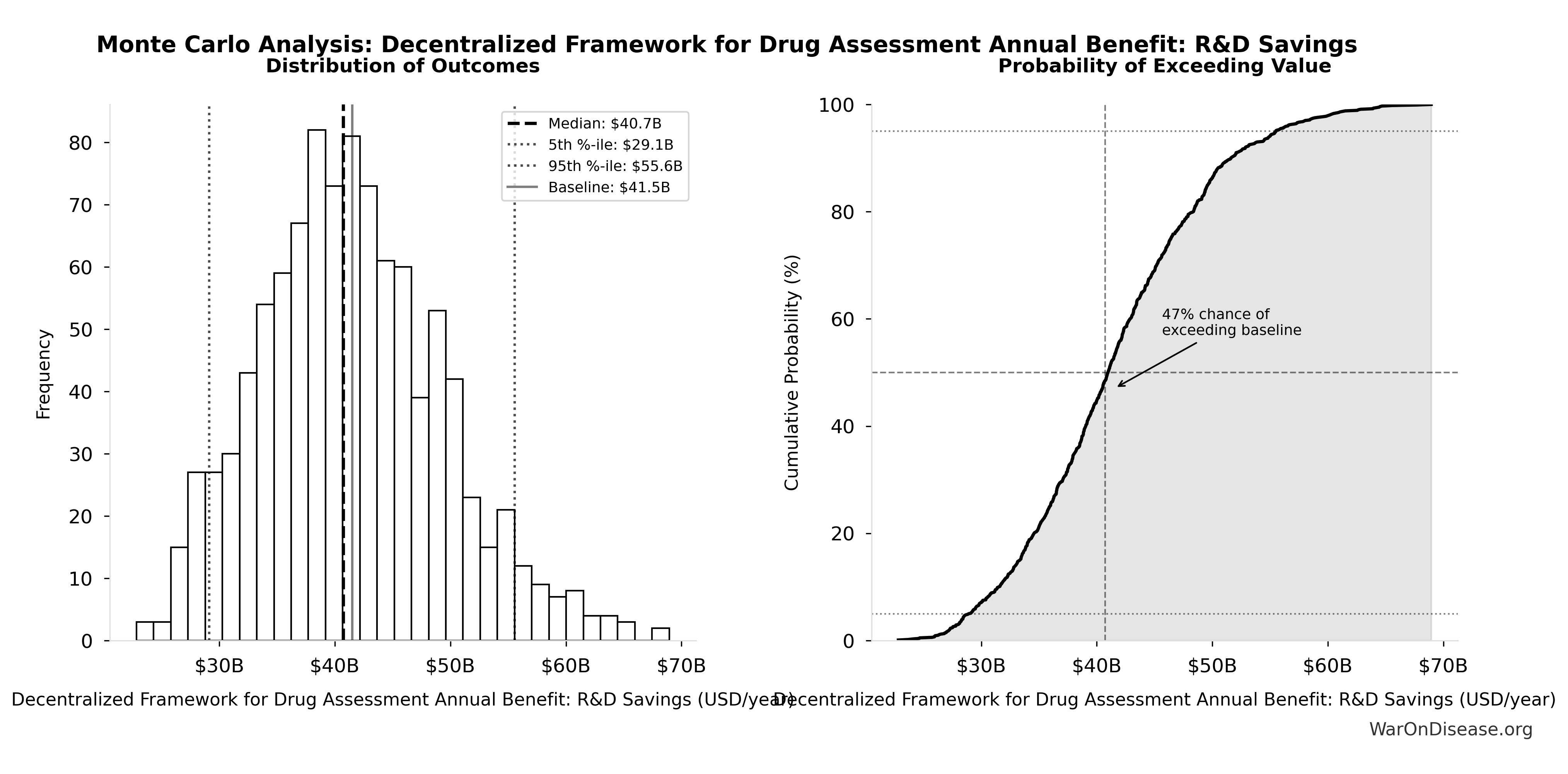
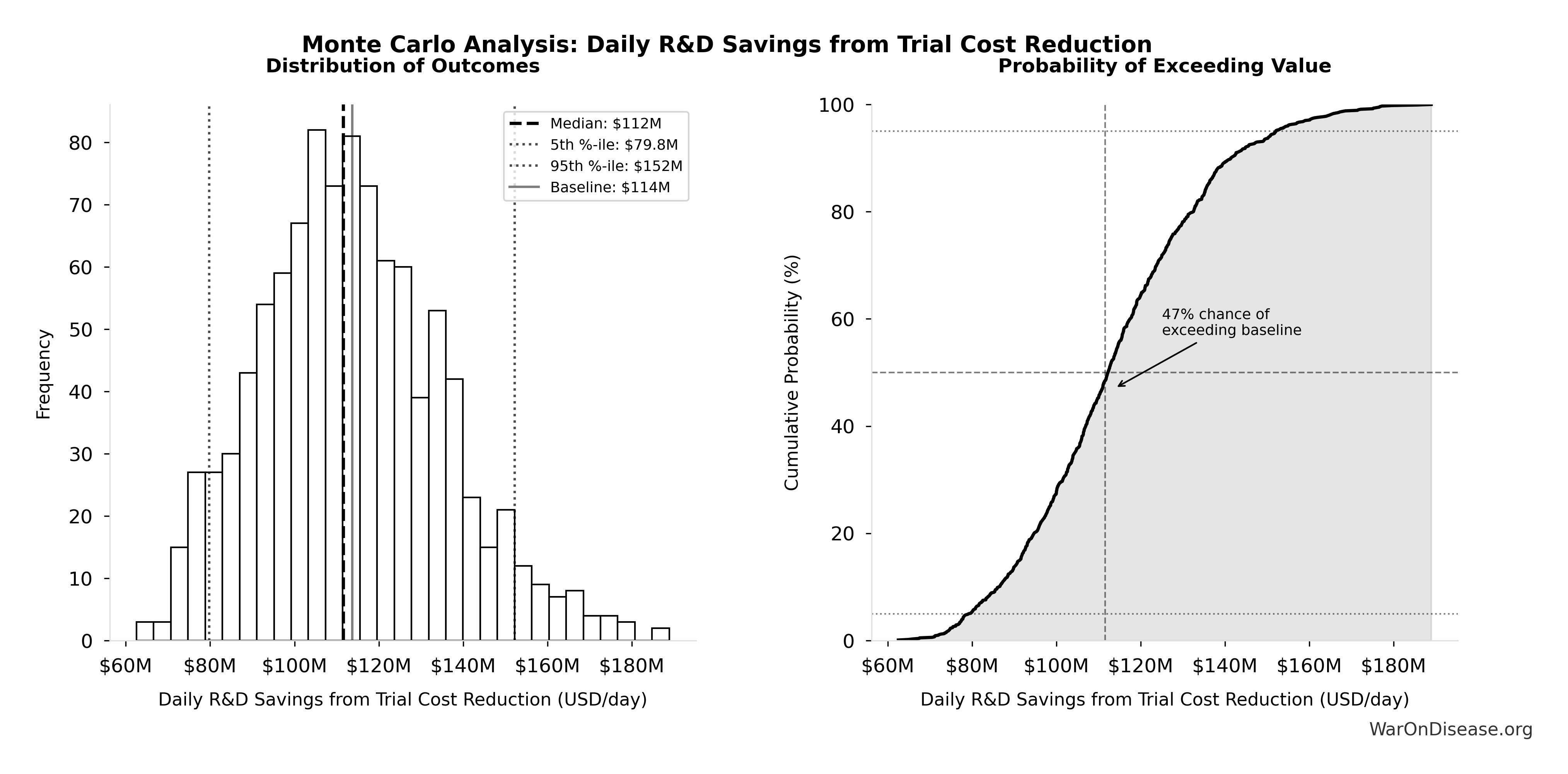
Monte Carlo Distribution
Simulation Results Summary: Decentralized Framework for Drug Assessment Annual Benefit: R&D Savings
| Statistic | Value |
|---|---|
| Baseline (deterministic) | $58.6B |
| Mean (expected value) | $58.8B |
| Median (50th percentile) | $57.8B |
| Standard Deviation | $7.66B |
| 90% Range (5th-95th percentile) | [$49.2B, $73.1B] |
The histogram shows the distribution of Decentralized Framework for Drug Assessment Annual Benefit: R&D Savings across 10,000 Monte Carlo simulations. The CDF (right) shows the probability of the outcome exceeding any given value, which is useful for risk assessment.
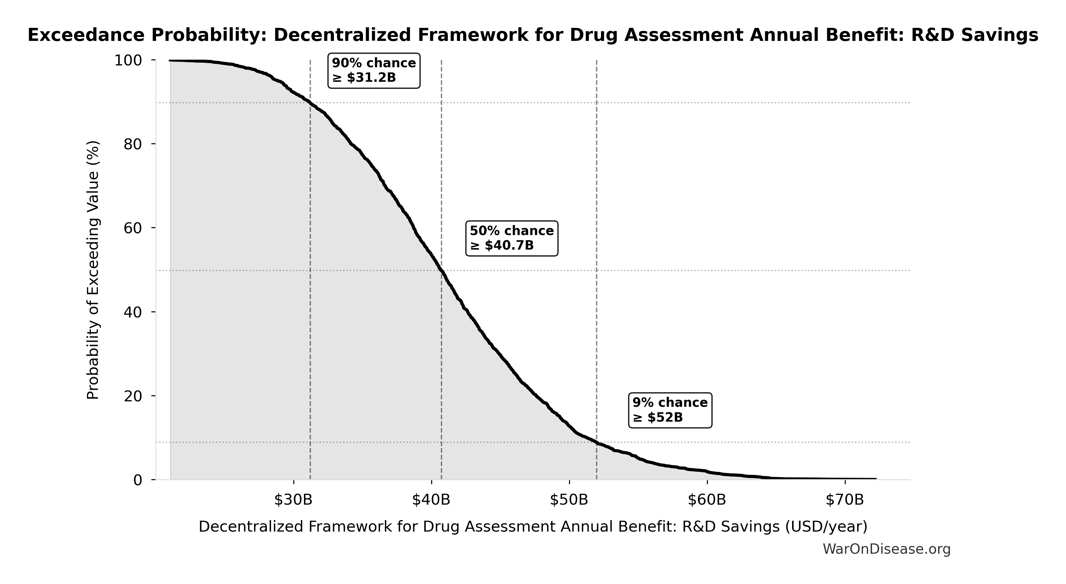
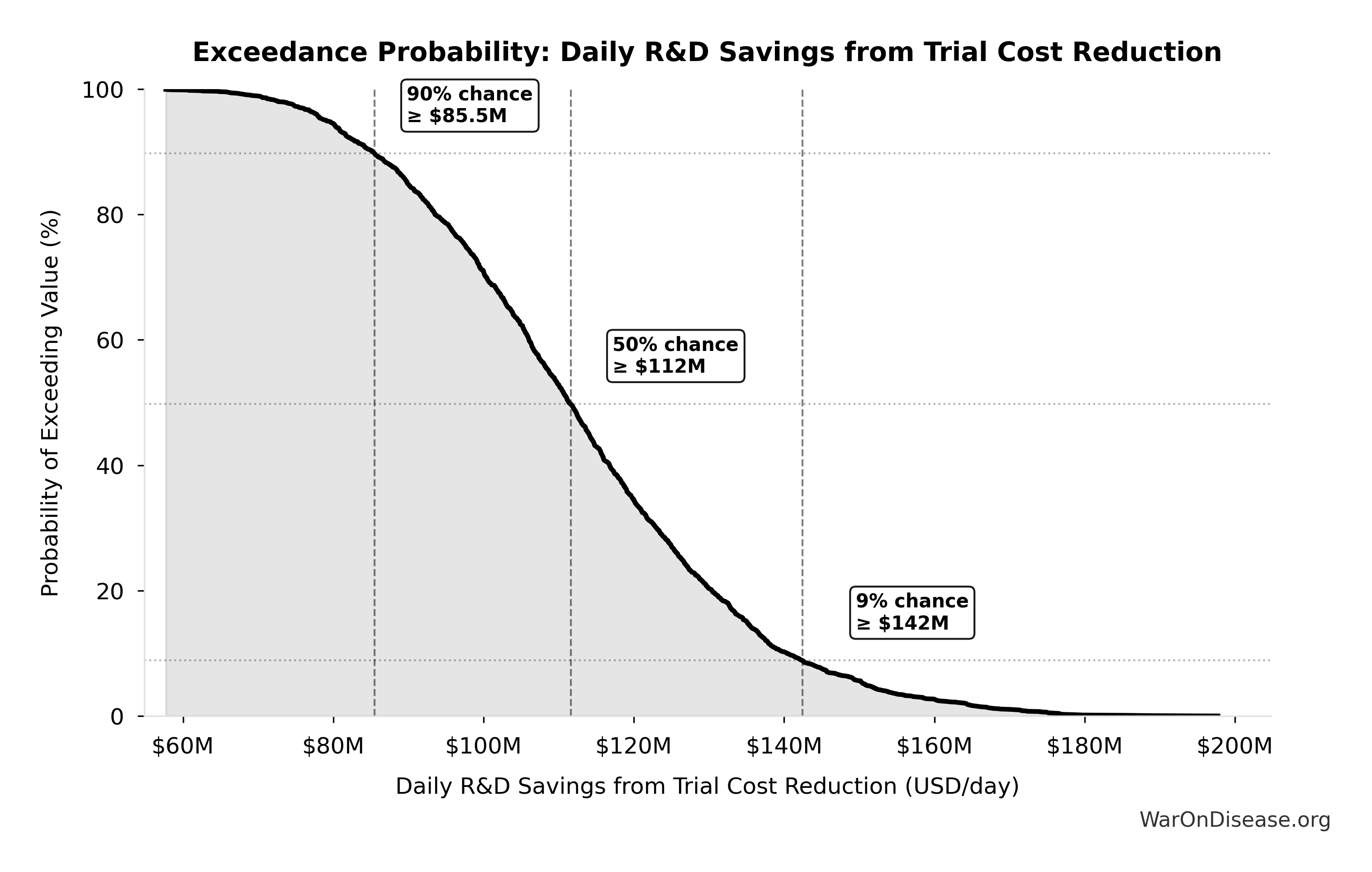
Exceedance Probability
This exceedance probability chart shows the likelihood that Decentralized Framework for Drug Assessment Annual Benefit: R&D Savings will exceed any given threshold. Higher curves indicate more favorable outcomes with greater certainty.
dFDA Direct Funding Cost per DALY: $0.842
Note📊 Details
Cost per DALY at direct funding level for the therapeutic space exploration period. Still highly cost-effective vs bed nets.
Inputs:
- dFDA Direct Funding NPV (Exploration Period) 🔢: $476B
- Total DALYs from Elimination of Efficacy Lag Plus Earlier Treatment Discovery from Higher Trial Throughput 🔢: 565 billion DALYs
\[ \begin{gathered} Cost_{direct,DALY} \\ = \frac{NPV_{direct}}{DALYs_{max}} \\ = \frac{\$476B}{565B} \\ = \$0.842 \end{gathered} \] where: \[ NPV_{direct} = Funding_{ann} \times \frac{1 - (1+r)^{-T}}{r} \] where: \[ \begin{gathered} T_{queue,dFDA} \\ = \frac{T_{queue,SQ}}{k_{capacity}} \\ = \frac{443}{12.3} \\ = 36 \end{gathered} \] where: \[ \begin{gathered} T_{queue,SQ} \\ = \frac{N_{untreated}}{Treatments_{new,ann}} \\ = \frac{6{,}650}{15} \\ = 443 \end{gathered} \] where: \[ \begin{gathered} N_{untreated} \\ = N_{rare} \times 0.95 \\ = 7{,}000 \times 0.95 \\ = 6{,}650 \end{gathered} \] where: \[ \begin{gathered} k_{capacity} \\ = \frac{N_{fundable,dFDA}}{Slots_{curr}} \\ = \frac{23.4M}{1.9M} \\ = 12.3 \end{gathered} \] where: \[ \begin{gathered} N_{fundable,dFDA} \\ = \frac{Subsidies_{dFDA,ann}}{Cost_{pragmatic,pt}} \\ = \frac{\$21.8B}{\$929} \\ = 23.4M \end{gathered} \] where: \[ \begin{gathered} Subsidies_{dFDA,ann} \\ = Funding_{dFDA,ann} - OPEX_{dFDA} \\ = \$21.8B - \$40M \\ = \$21.8B \end{gathered} \] where: \[ \begin{gathered} OPEX_{dFDA} \\ = Cost_{platform} + Cost_{staff} + Cost_{infra} \\ + Cost_{regulatory} + Cost_{community} \\ = \$15M + \$10M + \$8M + \$5M + \$2M \\ = \$40M \end{gathered} \] where: \[ \begin{gathered} DALYs_{max} \\ = DALYs_{global,ann} \times Pct_{avoid,DALY} \times T_{accel,max} \\ = 2.88B \times 92.6\% \times 212 \\ = 565B \end{gathered} \] where: \[ T_{accel,max} = T_{accel} + T_{lag} = 204 + 8.2 = 212 \] where: \[ \begin{gathered} T_{accel} \\ = T_{first,SQ} \times \left(1 - \frac{1}{k_{capacity}}\right) \\ = 222 \times \left(1 - \frac{1}{12.3}\right) \\ = 204 \end{gathered} \] where: \[ \begin{gathered} T_{first,SQ} \\ = T_{queue,SQ} \times 0.5 \\ = 443 \times 0.5 \\ = 222 \end{gathered} \] ~ Medium confidence
Sensitivity Analysis
Sensitivity Indices for dFDA Direct Funding Cost per DALY
Regression-based sensitivity showing which inputs explain the most variance in the output.
| Input Parameter | Sensitivity Coefficient | Interpretation |
|---|---|---|
| Total DALYs from Elimination of Efficacy Lag Plus Earlier Treatment Discovery from Higher Trial Throughput (DALYs) | -0.5173 | Strong driver |
| dFDA Direct Funding NPV (Exploration Period) (USD) | 0.4592 | Moderate driver |
Interpretation: Standardized coefficients show the change in output (in SD units) per 1 SD change in input. Values near ±1 indicate strong influence; values exceeding ±1 may occur with correlated inputs.
Monte Carlo Distribution
Simulation Results Summary: dFDA Direct Funding Cost per DALY
| Statistic | Value |
|---|---|
| Baseline (deterministic) | $0.842 |
| Mean (expected value) | $0.801 |
| Median (50th percentile) | $0.695 |
| Standard Deviation | $0.466 |
| 90% Range (5th-95th percentile) | [$0.242, $1.75] |
The histogram shows the distribution of dFDA Direct Funding Cost per DALY across 10,000 Monte Carlo simulations. The CDF (right) shows the probability of the outcome exceeding any given value, which is useful for risk assessment.
Exceedance Probability
This exceedance probability chart shows the likelihood that dFDA Direct Funding Cost per DALY will exceed any given threshold. Higher curves indicate more favorable outcomes with greater certainty.
dFDA Direct Funding NPV (Exploration Period): $476B
Note📊 Details
NPV of annual direct funding for the therapeutic space exploration period. Funding period equals exploration time (queue clearance years at given capacity multiplier). After exploration completes, the full timeline shift benefit is realized.
Inputs:
- dFDA Annual Trial Funding: $21.8B
- Standard Discount Rate for NPV Analysis: 3%
- dFDA Therapeutic Space Exploration Time 🔢: 36 years
\[ NPV_{direct} = Funding_{ann} \times \frac{1 - (1+r)^{-T}}{r} \]
✓ High confidence
Sensitivity Analysis
Sensitivity Indices for dFDA Direct Funding NPV (Exploration Period)
Regression-based sensitivity showing which inputs explain the most variance in the output.
| Input Parameter | Sensitivity Coefficient | Interpretation |
|---|---|---|
| dFDA Therapeutic Space Exploration Time (years) | 0.9444 | Strong driver |
Interpretation: Standardized coefficients show the change in output (in SD units) per 1 SD change in input. Values near ±1 indicate strong influence; values exceeding ±1 may occur with correlated inputs.
Monte Carlo Distribution
Simulation Results Summary: dFDA Direct Funding NPV (Exploration Period)
| Statistic | Value |
|---|---|
| Baseline (deterministic) | $476B |
| Mean (expected value) | $426B |
| Median (50th percentile) | $424B |
| Standard Deviation | $135B |
| 90% Range (5th-95th percentile) | [$211B, $652B] |
The histogram shows the distribution of dFDA Direct Funding NPV (Exploration Period) across 10,000 Monte Carlo simulations. The CDF (right) shows the probability of the outcome exceeding any given value, which is useful for risk assessment.
Exceedance Probability
This exceedance probability chart shows the likelihood that dFDA Direct Funding NPV (Exploration Period) will exceed any given threshold. Higher curves indicate more favorable outcomes with greater certainty.
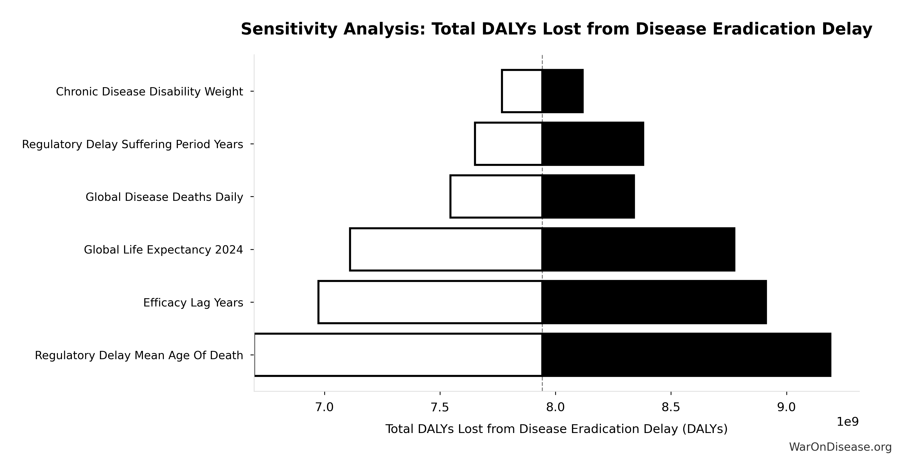
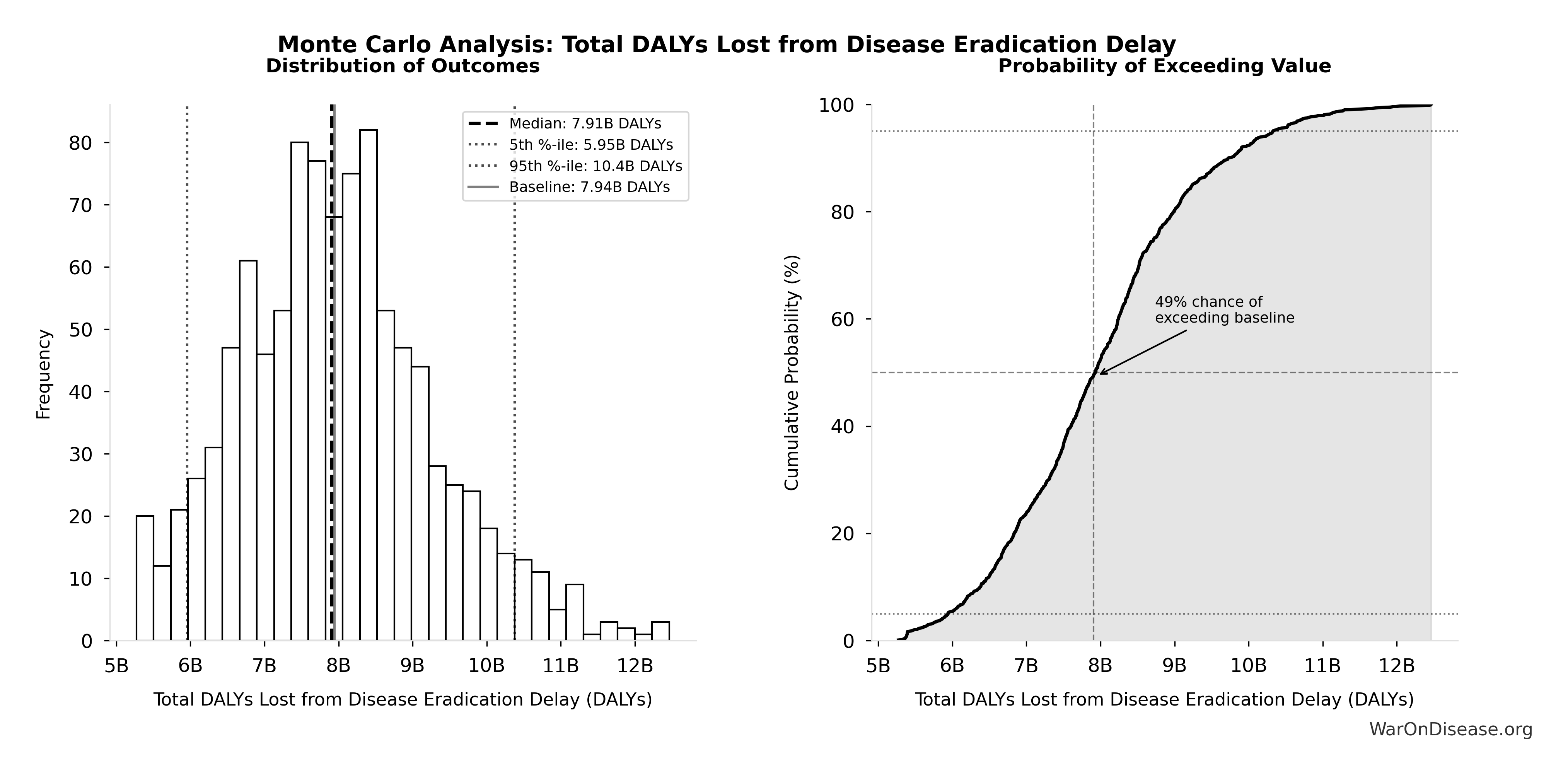
Total DALYs Lost from Disease Eradication Delay: 7.94 billion DALYs
Note📊 Details
Total Disability-Adjusted Life Years lost from disease eradication delay (PRIMARY estimate)
Inputs:
- Years of Life Lost from Disease Eradication Delay 🔢: 7.07 billion years
- Years Lived with Disability During Disease Eradication Delay 🔢: 873 million years
\[ DALYs_{lag} = YLL_{lag} + YLD_{lag} = 7.07B + 873M = 7.94B \] where: \[ \begin{gathered} YLL_{lag} \\ = Deaths_{lag} \times (LE_{global} - Age_{death,delay}) \\ = 416M \times (79 - 62) \\ = 7.07B \end{gathered} \] where: \[ \begin{gathered} Deaths_{lag} \\ = T_{lag} \times Deaths_{disease,daily} \times 338 \\ = 8.2 \times 150{,}000 \times 338 \\ = 416M \end{gathered} \] where: \[ \begin{gathered} YLD_{lag} \\ = Deaths_{lag} \times T_{suffering} \times DW_{chronic} \\ = 416M \times 6 \times 0.35 \\ = 873M \end{gathered} \] ~ Medium confidence
Sensitivity Analysis
Sensitivity Indices for Total DALYs Lost from Disease Eradication Delay
Regression-based sensitivity showing which inputs explain the most variance in the output.
| Input Parameter | Sensitivity Coefficient | Interpretation |
|---|---|---|
| Years of Life Lost from Disease Eradication Delay (years) | 0.7043 | Strong driver |
| Years Lived with Disability During Disease Eradication Delay (years) | 0.3107 | Moderate driver |
Interpretation: Standardized coefficients show the change in output (in SD units) per 1 SD change in input. Values near ±1 indicate strong influence; values exceeding ±1 may occur with correlated inputs.
Monte Carlo Distribution
Simulation Results Summary: Total DALYs Lost from Disease Eradication Delay
| Statistic | Value |
|---|---|
| Baseline (deterministic) | 7.94 billion |
| Mean (expected value) | 8.05 billion |
| Median (50th percentile) | 7.89 billion |
| Standard Deviation | 2.31 billion |
| 90% Range (5th-95th percentile) | [4.43 billion, 12.1 billion] |
The histogram shows the distribution of Total DALYs Lost from Disease Eradication Delay across 10,000 Monte Carlo simulations. The CDF (right) shows the probability of the outcome exceeding any given value, which is useful for risk assessment.
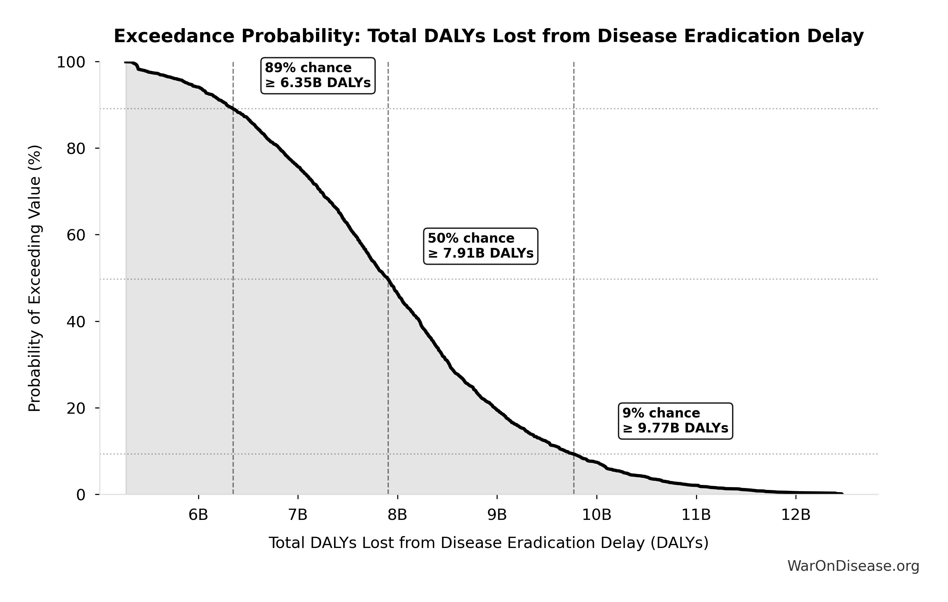
Exceedance Probability
This exceedance probability chart shows the likelihood that Total DALYs Lost from Disease Eradication Delay will exceed any given threshold. Higher curves indicate more favorable outcomes with greater certainty.
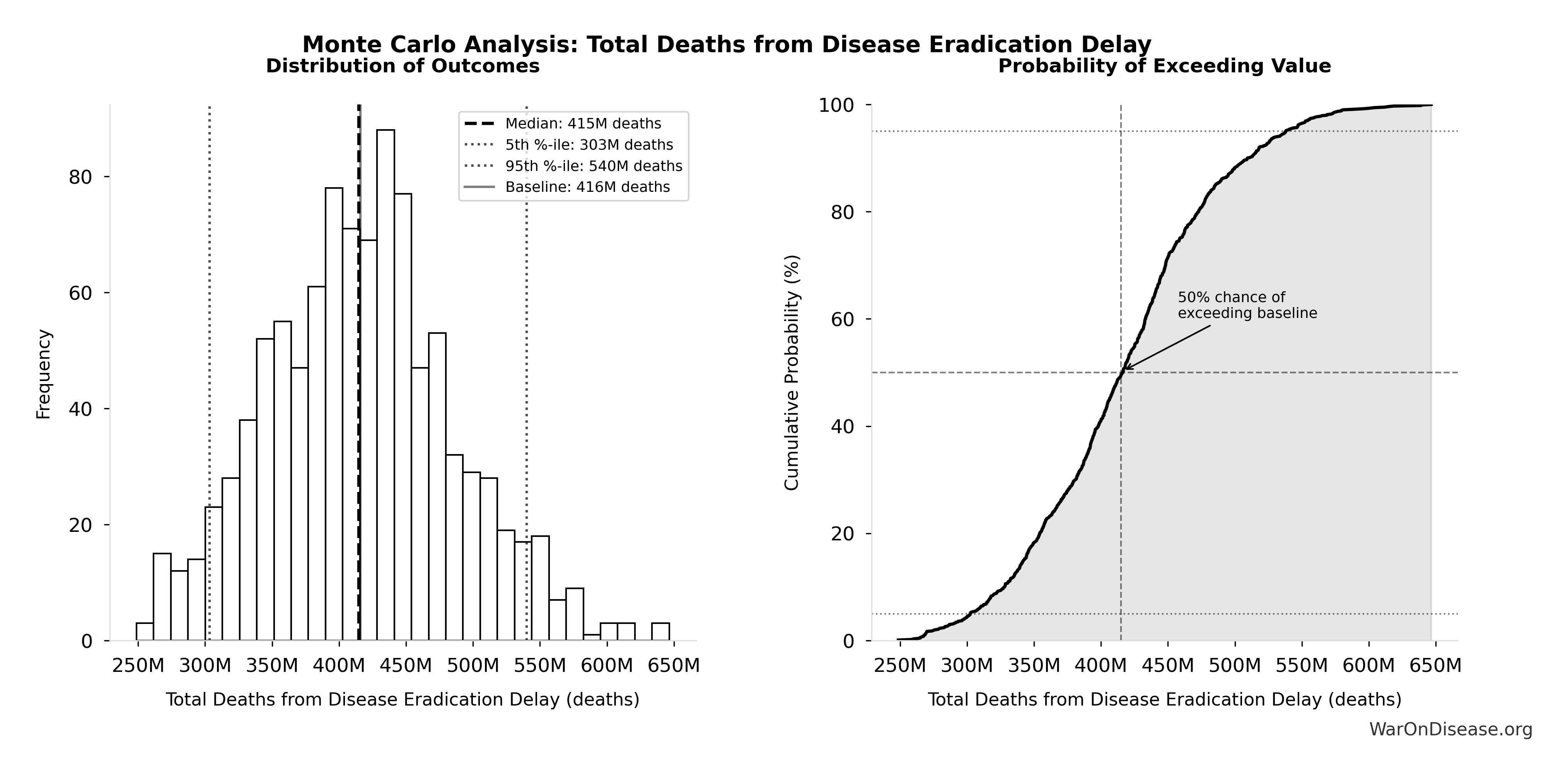
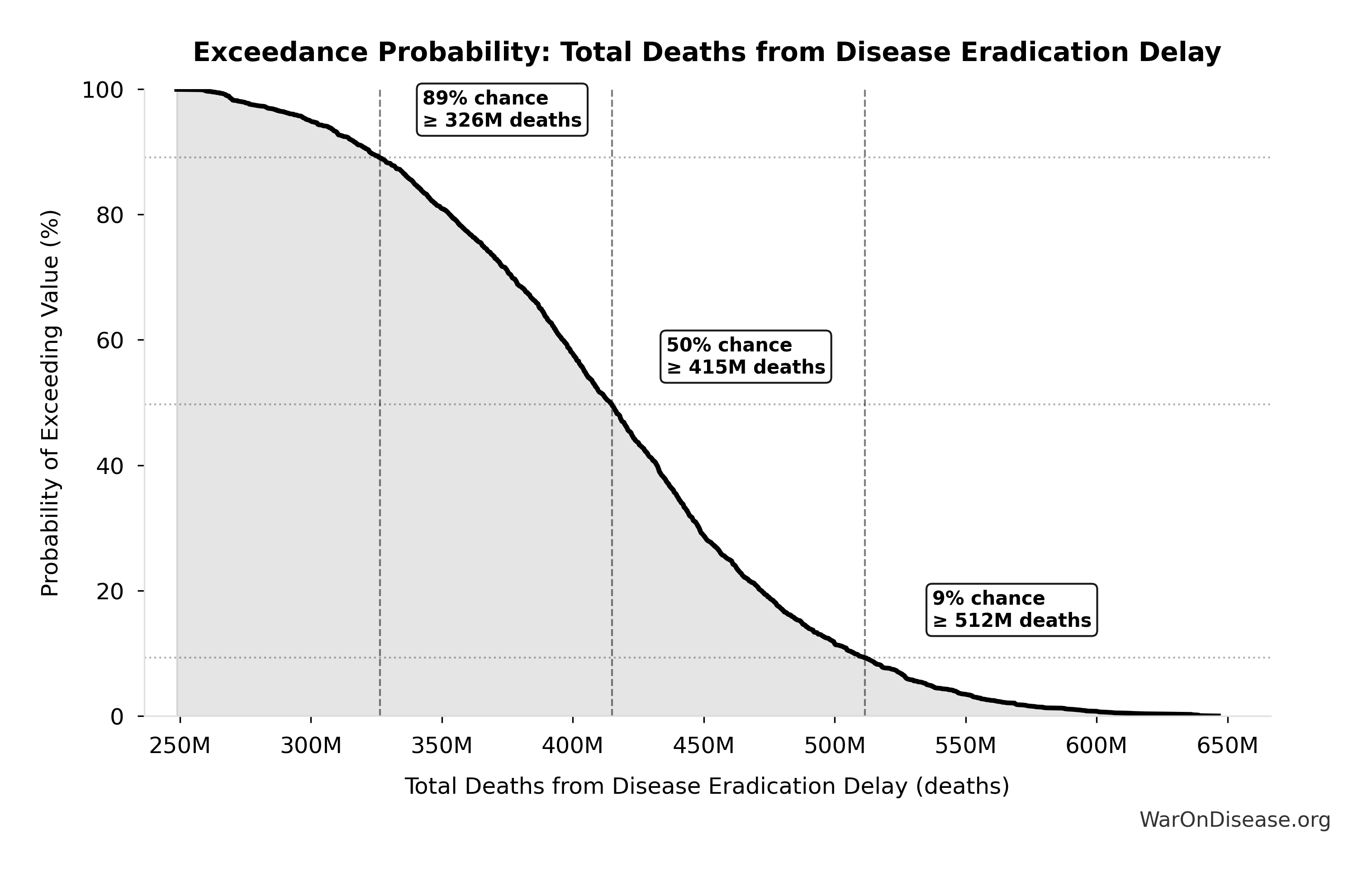
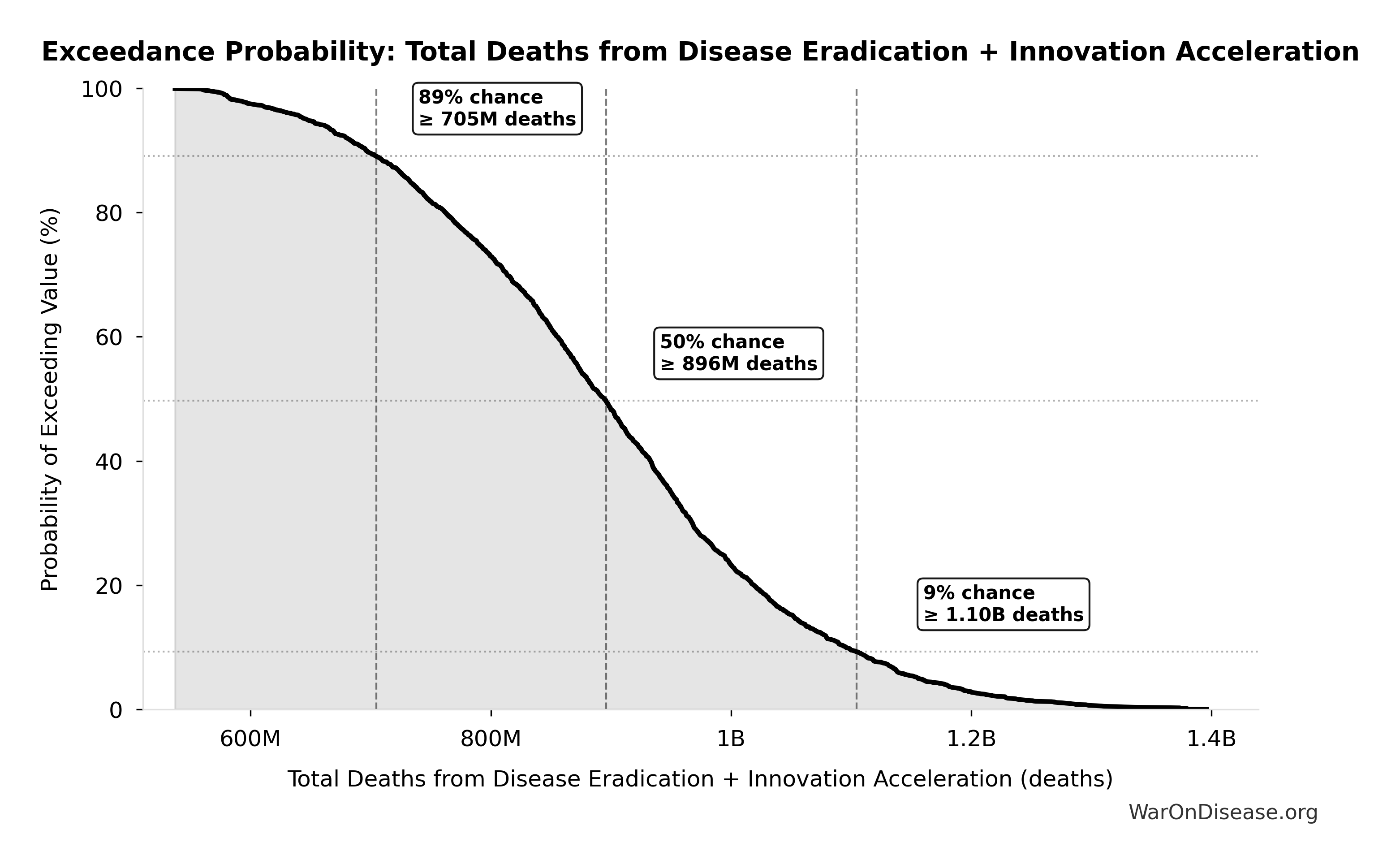
Total Deaths from Disease Eradication Delay: 416 million deaths
Note📊 Details
Total eventually avoidable deaths from delaying disease eradication by 8.2 years (PRIMARY estimate, conservative). Excludes fundamentally unavoidable deaths (primarily accidents ~7.9%).
Inputs:
- Regulatory Delay for Efficacy Testing Post-Safety Verification 📊: 8.2 years (SE: ±2 years)
- Global Daily Deaths from Disease and Aging 📊: 150 thousand deaths/day (SE: ±7.5 thousand deaths/day)
\[ \begin{gathered} Deaths_{lag} \\ = T_{lag} \times Deaths_{disease,daily} \times 338 \\ = 8.2 \times 150{,}000 \times 338 \\ = 416M \end{gathered} \]
~ Medium confidence
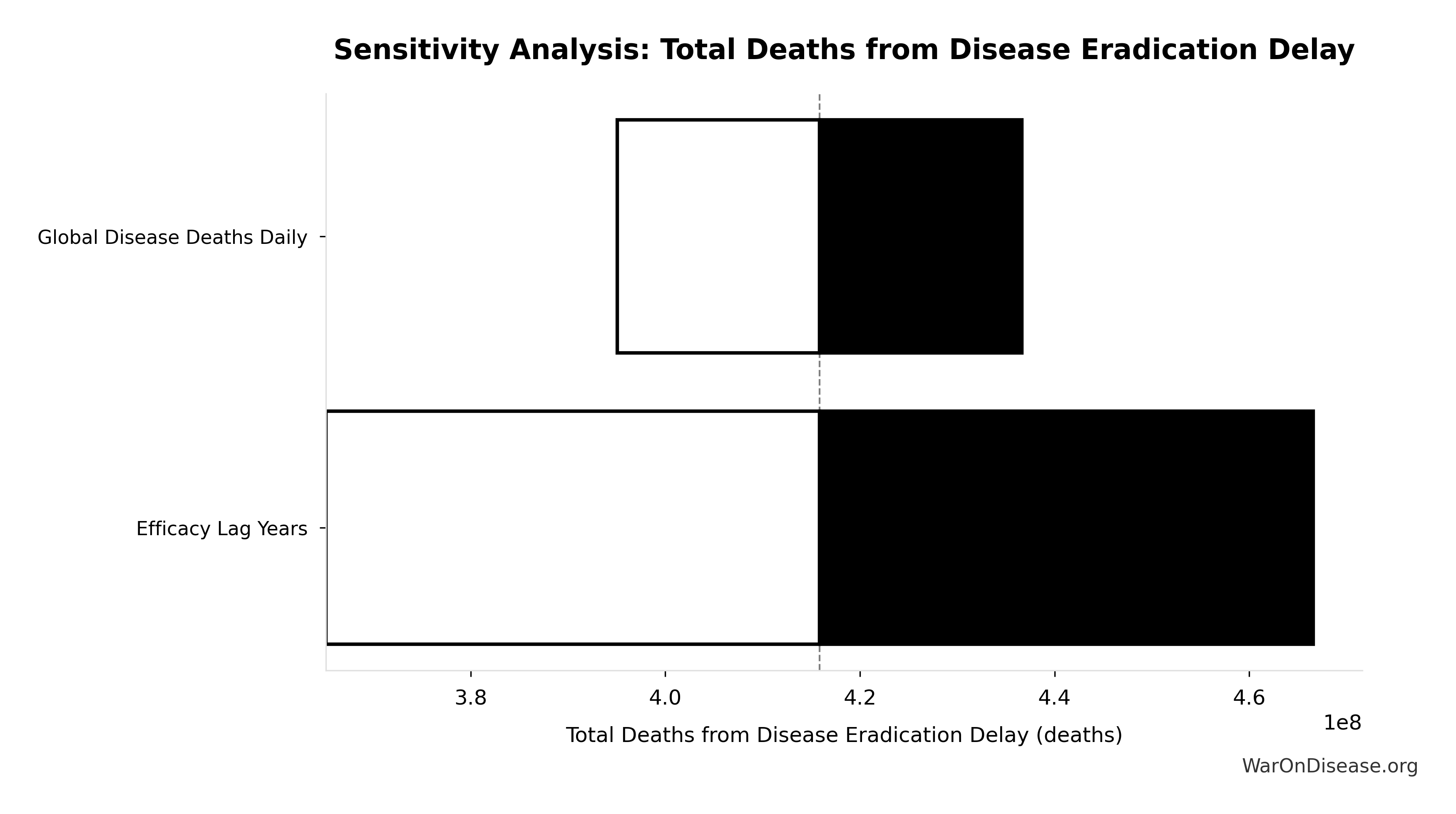
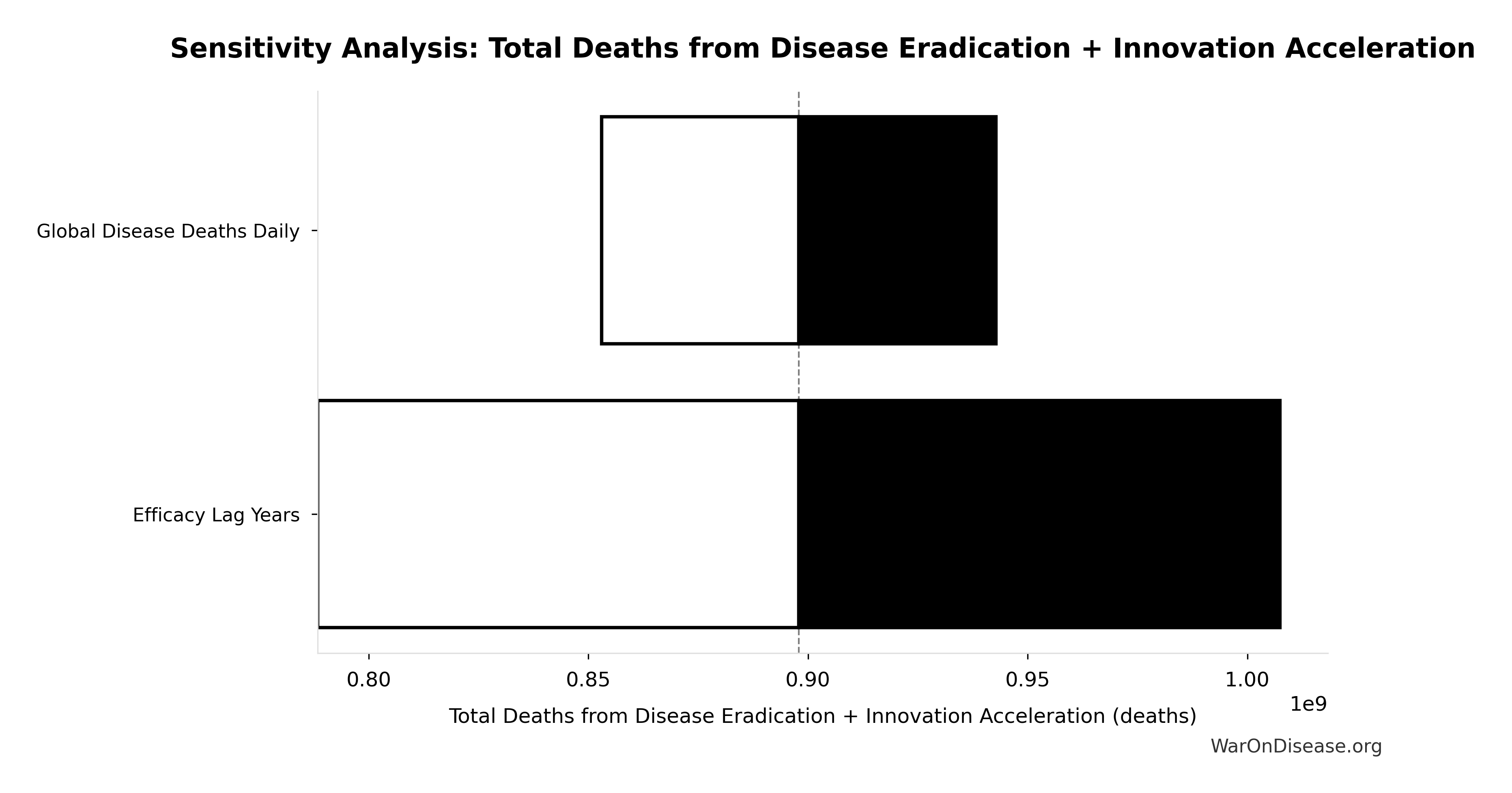
Sensitivity Analysis
Sensitivity Indices for Total Deaths from Disease Eradication Delay
Regression-based sensitivity showing which inputs explain the most variance in the output.
| Input Parameter | Sensitivity Coefficient | Interpretation |
|---|---|---|
| Regulatory Delay for Efficacy Testing Post-Safety Verification (years) | 1.1404 | Strong driver |
| Global Daily Deaths from Disease and Aging (deaths/day) | -0.1422 | Weak driver |
Interpretation: Standardized coefficients show the change in output (in SD units) per 1 SD change in input. Values near ±1 indicate strong influence; values exceeding ±1 may occur with correlated inputs.
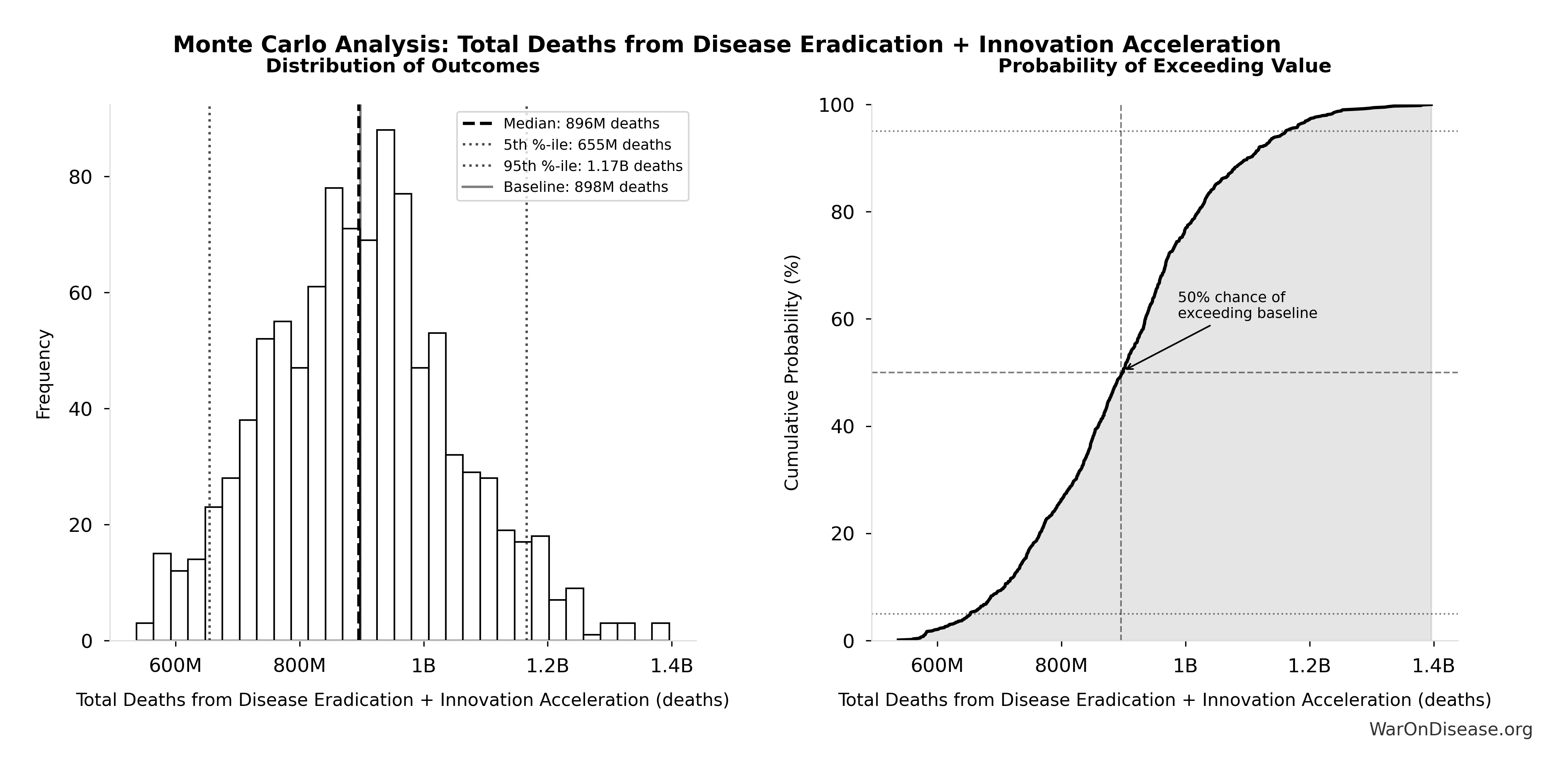
Monte Carlo Distribution
Simulation Results Summary: Total Deaths from Disease Eradication Delay
| Statistic | Value |
|---|---|
| Baseline (deterministic) | 416 million |
| Mean (expected value) | 420 million |
| Median (50th percentile) | 414 million |
| Standard Deviation | 122 million |
| 90% Range (5th-95th percentile) | [225 million, 630 million] |
The histogram shows the distribution of Total Deaths from Disease Eradication Delay across 10,000 Monte Carlo simulations. The CDF (right) shows the probability of the outcome exceeding any given value, which is useful for risk assessment.
Exceedance Probability
This exceedance probability chart shows the likelihood that Total Deaths from Disease Eradication Delay will exceed any given threshold. Higher curves indicate more favorable outcomes with greater certainty.
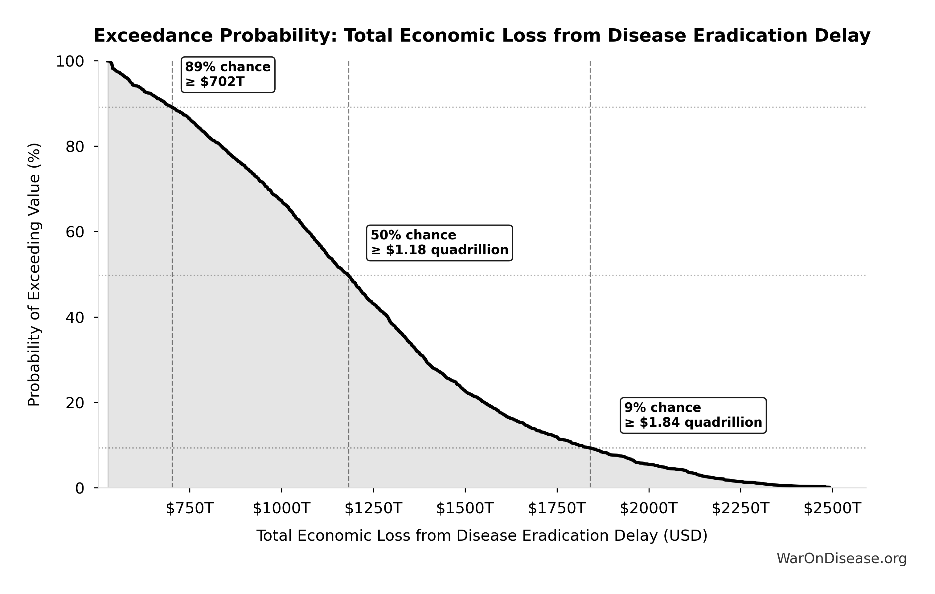
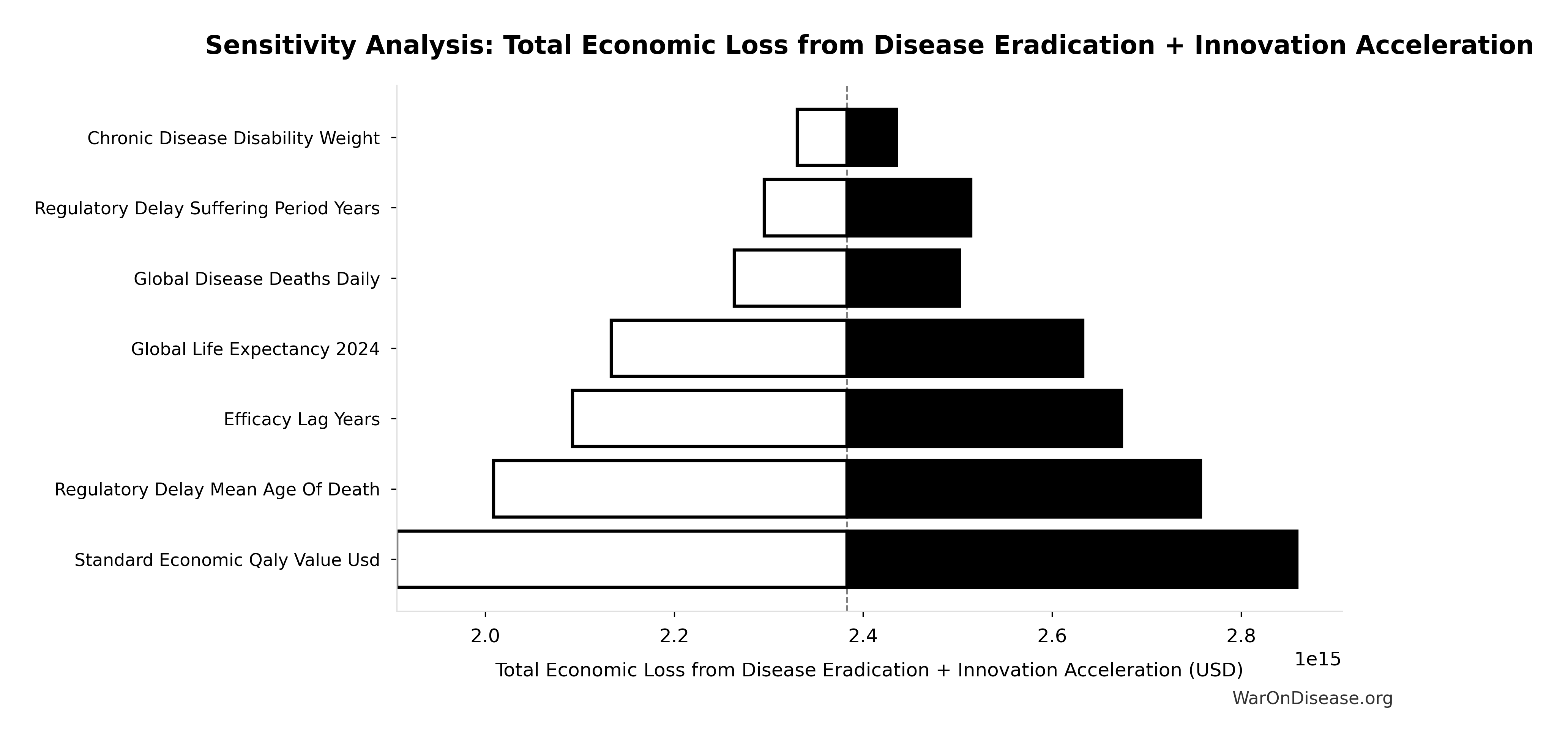
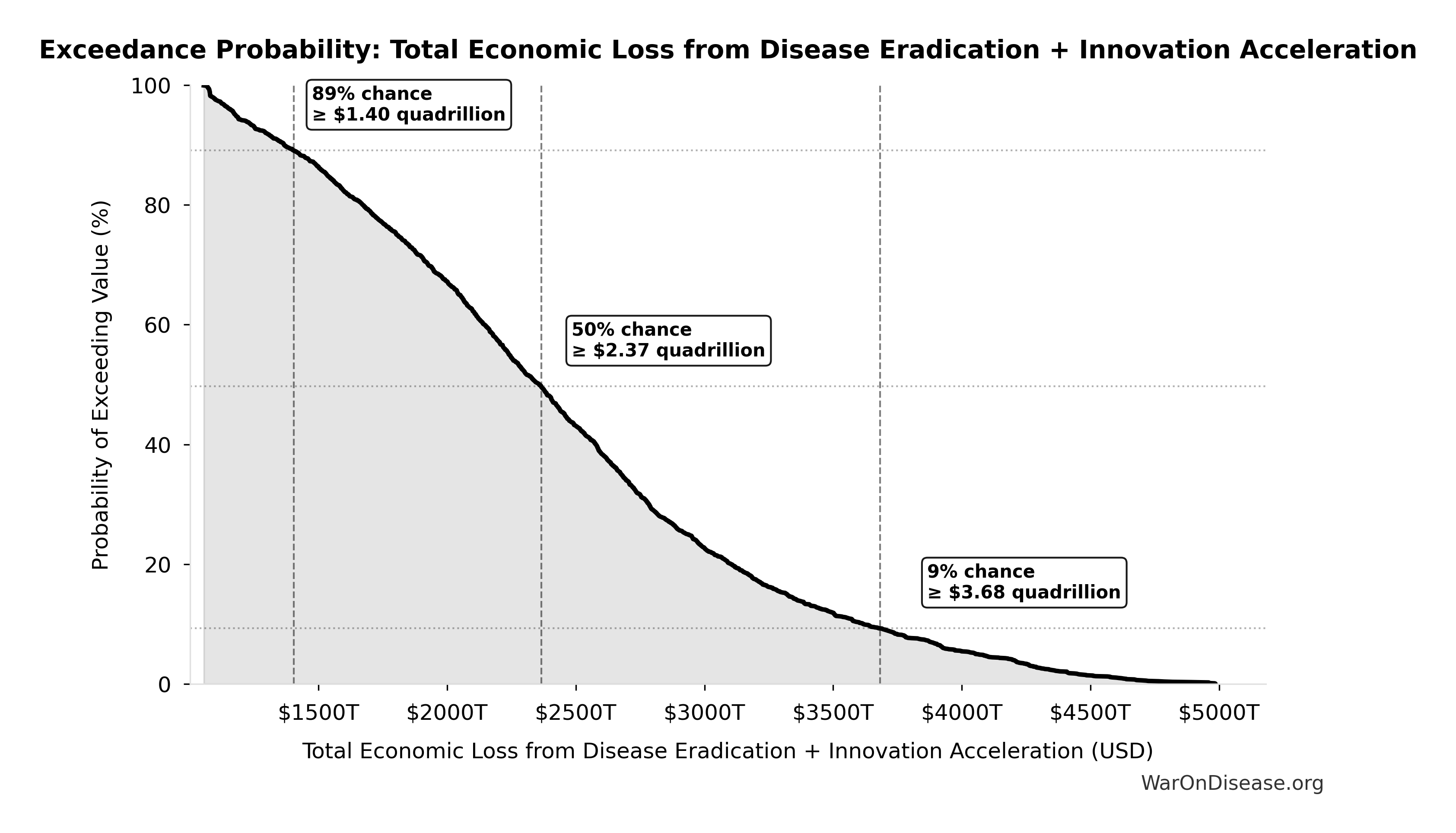
Total Economic Loss from Disease Eradication Delay: $1.19 quadrillion
Note📊 Details
Total economic loss from delaying disease eradication by 8.2 years (PRIMARY estimate, 2024 USD). Values global DALYs at standardized US/International normative rate ($150k) rather than local ability-to-pay, representing the full human capital loss.
Inputs:
- Total DALYs Lost from Disease Eradication Delay 🔢: 7.94 billion DALYs
- Standard Economic Value per QALY 📊: $150K (SE: ±$30K)
\[ \begin{gathered} Value_{lag} \\ = DALYs_{lag} \times Value_{QALY} \\ = 7.94B \times \$150K \\ = \$1190T \end{gathered} \] where: \[ DALYs_{lag} = YLL_{lag} + YLD_{lag} = 7.07B + 873M = 7.94B \] where: \[ \begin{gathered} YLL_{lag} \\ = Deaths_{lag} \times (LE_{global} - Age_{death,delay}) \\ = 416M \times (79 - 62) \\ = 7.07B \end{gathered} \] where: \[ \begin{gathered} Deaths_{lag} \\ = T_{lag} \times Deaths_{disease,daily} \times 338 \\ = 8.2 \times 150{,}000 \times 338 \\ = 416M \end{gathered} \] where: \[ \begin{gathered} YLD_{lag} \\ = Deaths_{lag} \times T_{suffering} \times DW_{chronic} \\ = 416M \times 6 \times 0.35 \\ = 873M \end{gathered} \] ~ Medium confidence
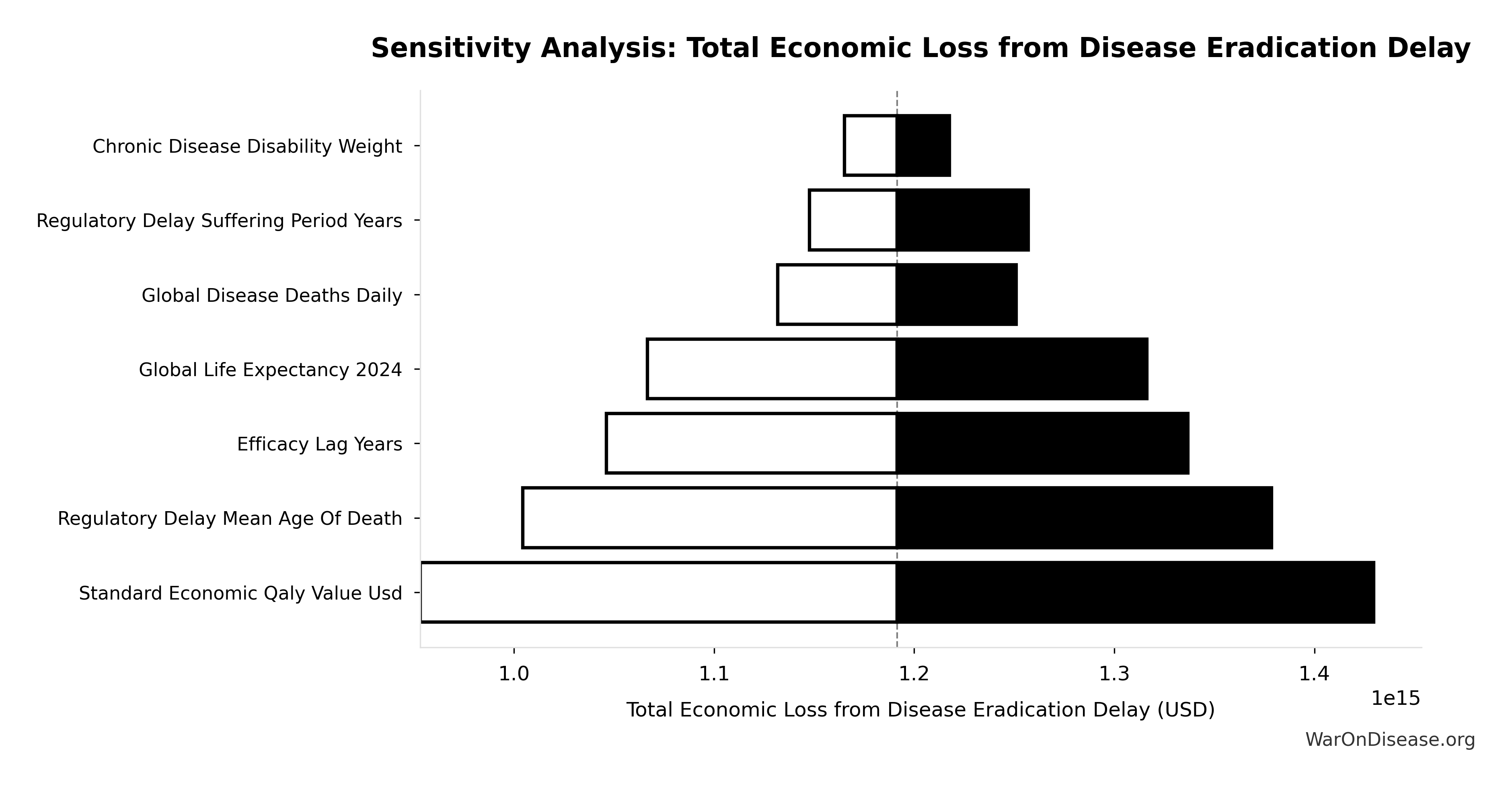
Sensitivity Analysis
Sensitivity Indices for Total Economic Loss from Disease Eradication Delay
Regression-based sensitivity showing which inputs explain the most variance in the output.
| Input Parameter | Sensitivity Coefficient | Interpretation |
|---|---|---|
| Total DALYs Lost from Disease Eradication Delay (DALYs) | 1.0671 | Strong driver |
| Standard Economic Value per QALY (USD/QALY) | -0.0733 | Minimal effect |
Interpretation: Standardized coefficients show the change in output (in SD units) per 1 SD change in input. Values near ±1 indicate strong influence; values exceeding ±1 may occur with correlated inputs.
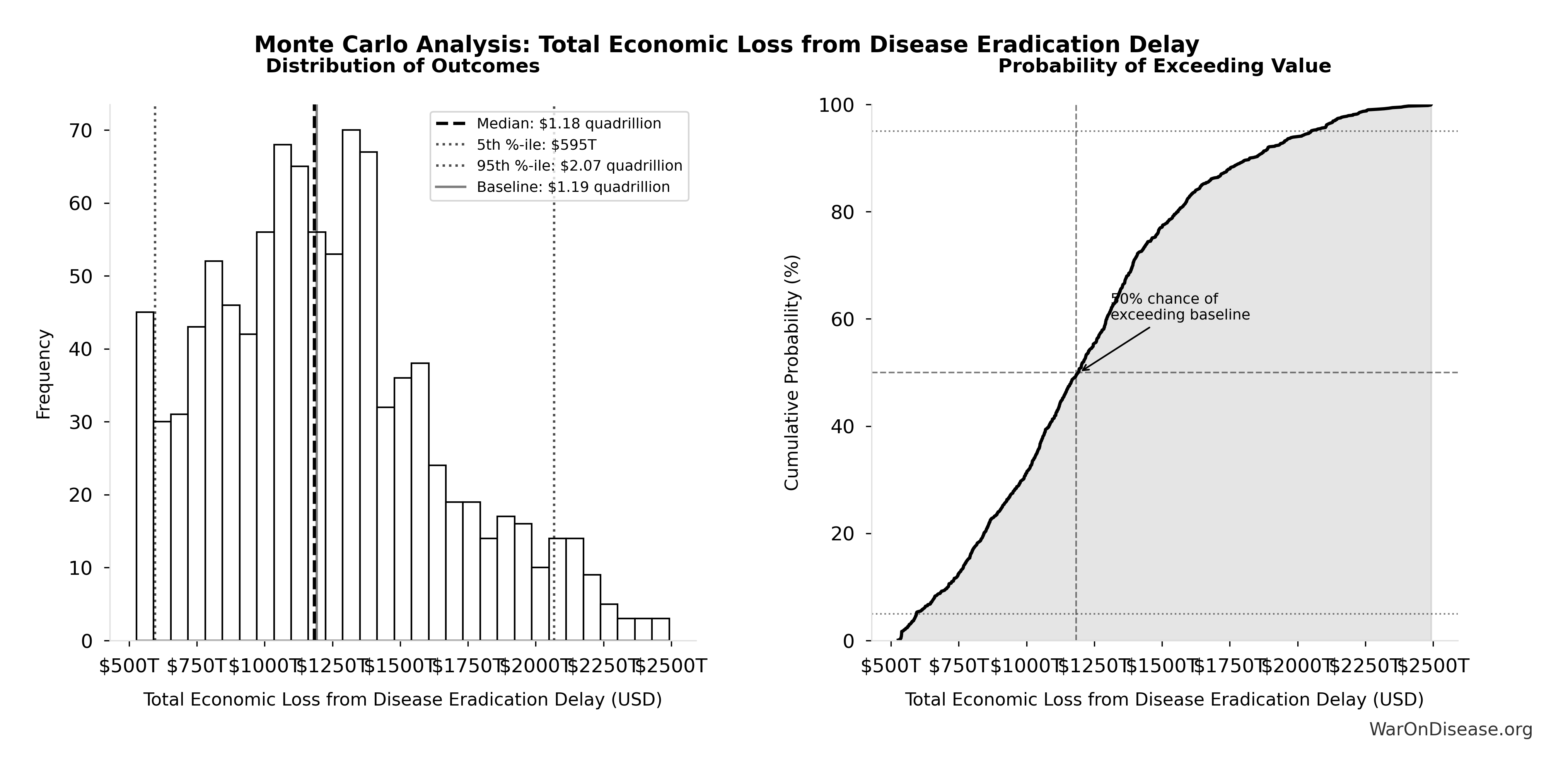
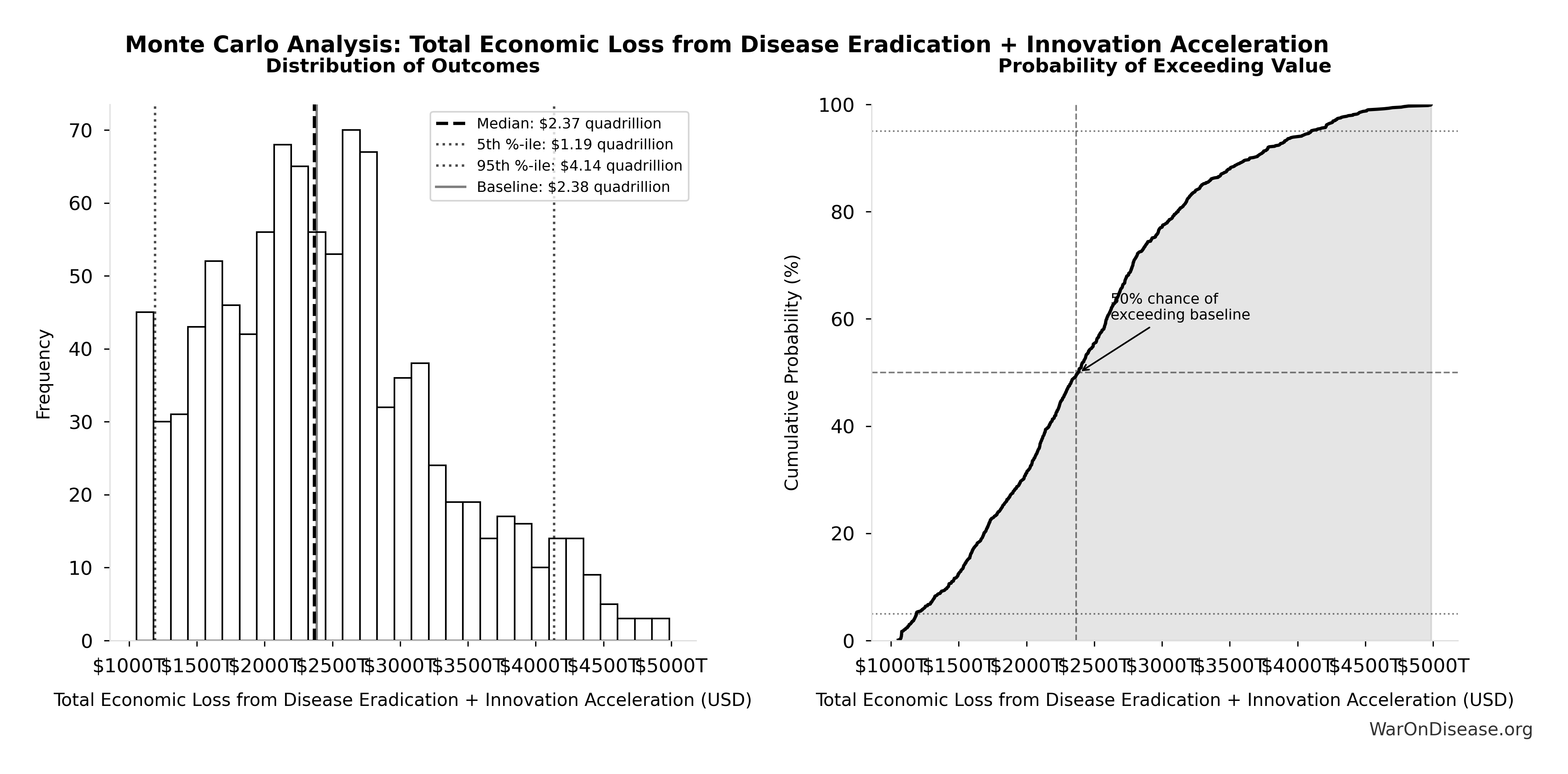
Monte Carlo Distribution
Simulation Results Summary: Total Economic Loss from Disease Eradication Delay
| Statistic | Value |
|---|---|
| Baseline (deterministic) | $1.19 quadrillion |
| Mean (expected value) | $1.27 quadrillion |
| Median (50th percentile) | $1.18 quadrillion |
| Standard Deviation | $581T |
| 90% Range (5th-95th percentile) | [$443T, $2.41 quadrillion] |
The histogram shows the distribution of Total Economic Loss from Disease Eradication Delay across 10,000 Monte Carlo simulations. The CDF (right) shows the probability of the outcome exceeding any given value, which is useful for risk assessment.
Exceedance Probability
This exceedance probability chart shows the likelihood that Total Economic Loss from Disease Eradication Delay will exceed any given threshold. Higher curves indicate more favorable outcomes with greater certainty.
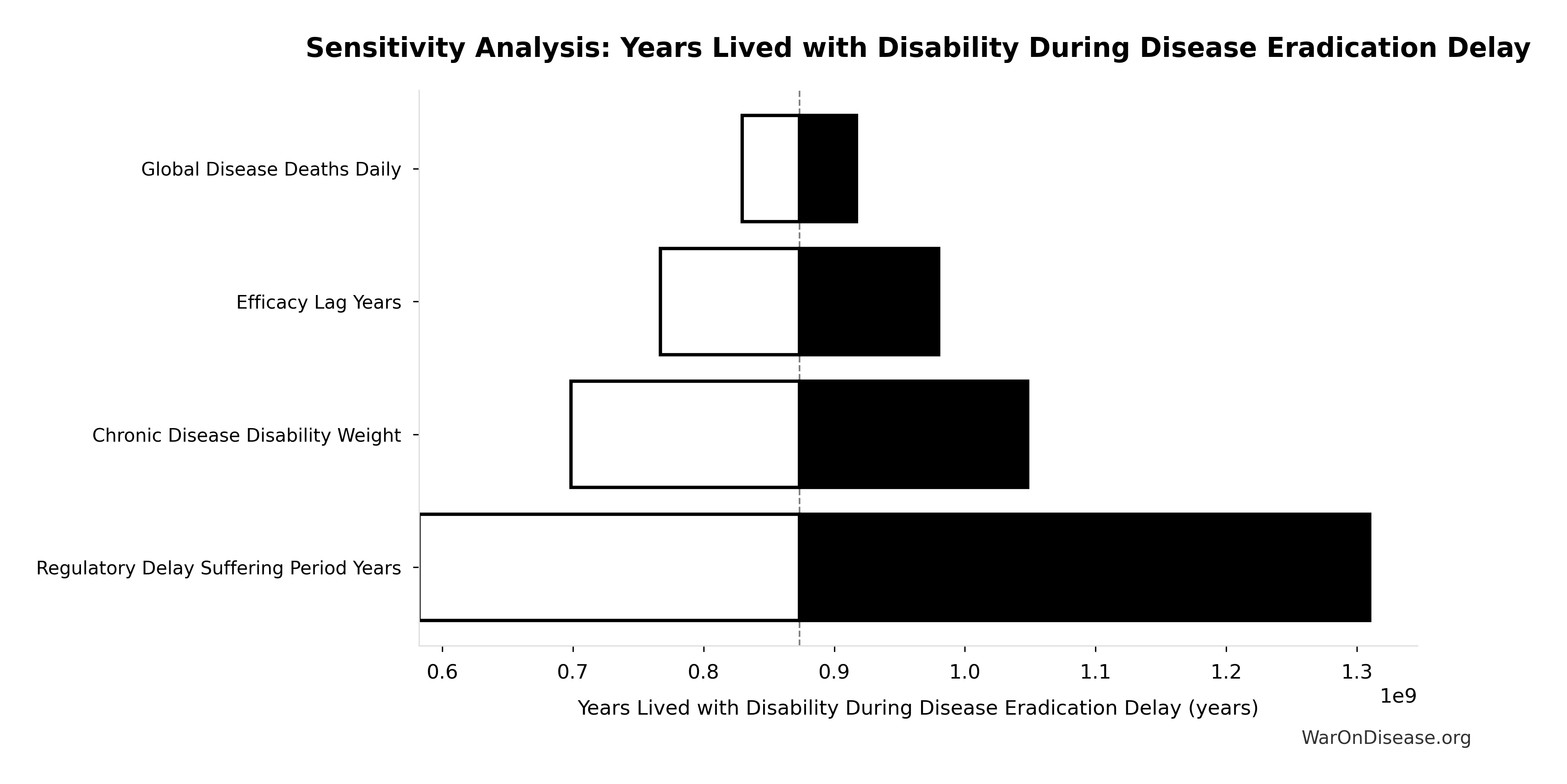
Years Lived with Disability During Disease Eradication Delay: 873 million years
Note📊 Details
Years Lived with Disability during disease eradication delay (PRIMARY estimate)
Inputs:
- Total Deaths from Disease Eradication Delay 🔢: 416 million deaths
- Pre-Death Suffering Period During Post-Safety Efficacy Delay 📊: 6 years (95% CI: 4 years - 9 years)
- Disability Weight for Untreated Chronic Conditions 📊: 0.35 weight (SE: ±0.07 weight)
\[ \begin{gathered} YLD_{lag} \\ = Deaths_{lag} \times T_{suffering} \times DW_{chronic} \\ = 416M \times 6 \times 0.35 \\ = 873M \end{gathered} \] where: \[ \begin{gathered} Deaths_{lag} \\ = T_{lag} \times Deaths_{disease,daily} \times 338 \\ = 8.2 \times 150{,}000 \times 338 \\ = 416M \end{gathered} \] ~ Medium confidence
Sensitivity Analysis
Sensitivity Indices for Years Lived with Disability During Disease Eradication Delay
Regression-based sensitivity showing which inputs explain the most variance in the output.
| Input Parameter | Sensitivity Coefficient | Interpretation |
|---|---|---|
| Pre-Death Suffering Period During Post-Safety Efficacy Delay (years) | 2.0883 | Strong driver |
| Disability Weight for Untreated Chronic Conditions (weight) | -0.9003 | Strong driver |
| Total Deaths from Disease Eradication Delay (deaths) | -0.2255 | Weak driver |
Interpretation: Standardized coefficients show the change in output (in SD units) per 1 SD change in input. Values near ±1 indicate strong influence; values exceeding ±1 may occur with correlated inputs.
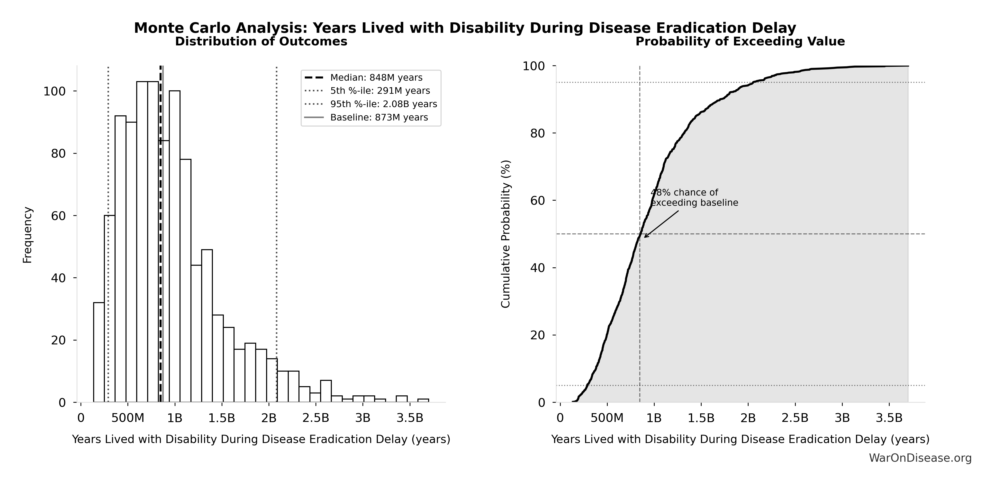
Monte Carlo Distribution
Simulation Results Summary: Years Lived with Disability During Disease Eradication Delay
| Statistic | Value |
|---|---|
| Baseline (deterministic) | 873 million |
| Mean (expected value) | 1.02 billion |
| Median (50th percentile) | 846 million |
| Standard Deviation | 716 million |
| 90% Range (5th-95th percentile) | [217 million, 2.43 billion] |
The histogram shows the distribution of Years Lived with Disability During Disease Eradication Delay across 10,000 Monte Carlo simulations. The CDF (right) shows the probability of the outcome exceeding any given value, which is useful for risk assessment.
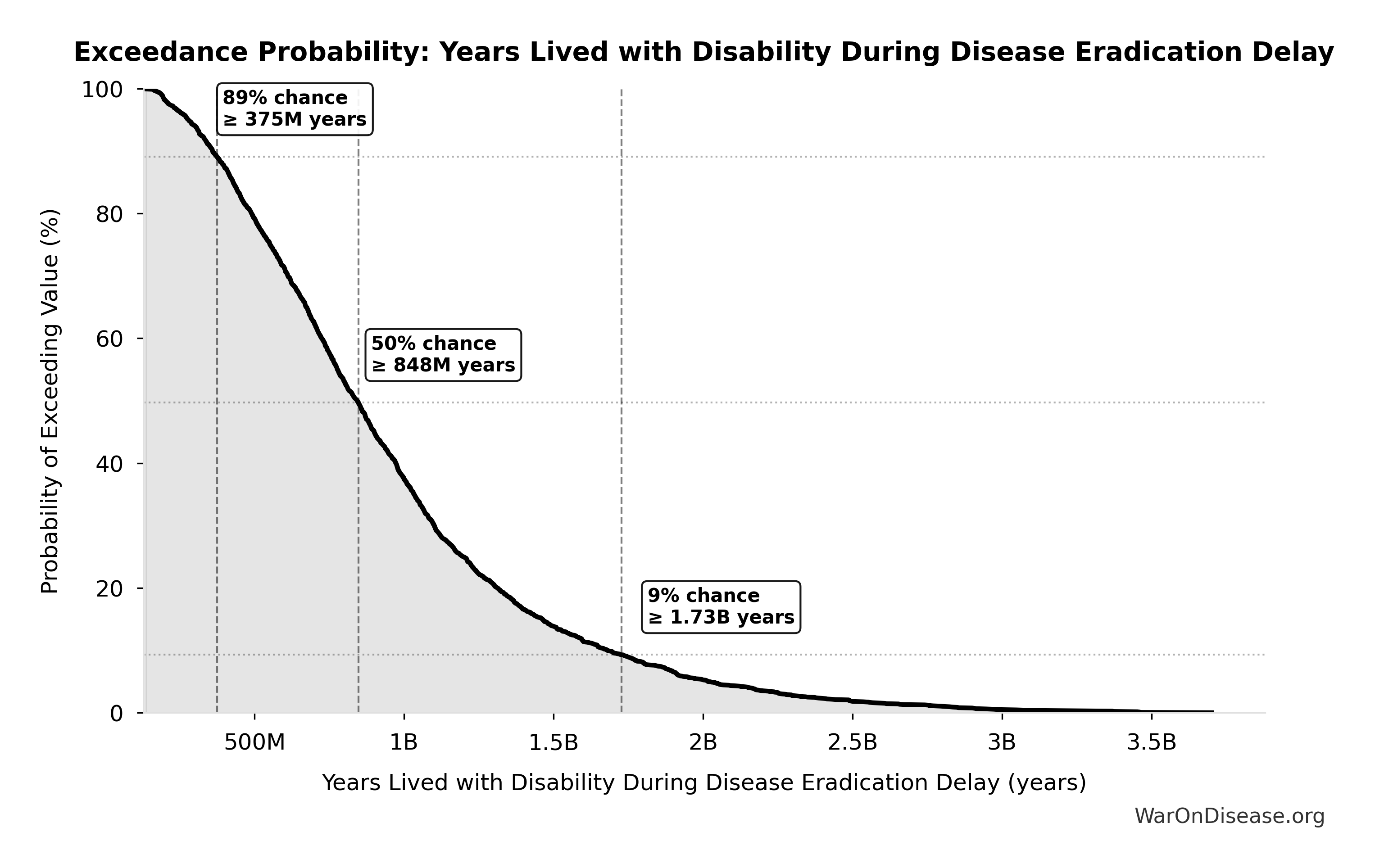
Exceedance Probability
This exceedance probability chart shows the likelihood that Years Lived with Disability During Disease Eradication Delay will exceed any given threshold. Higher curves indicate more favorable outcomes with greater certainty.
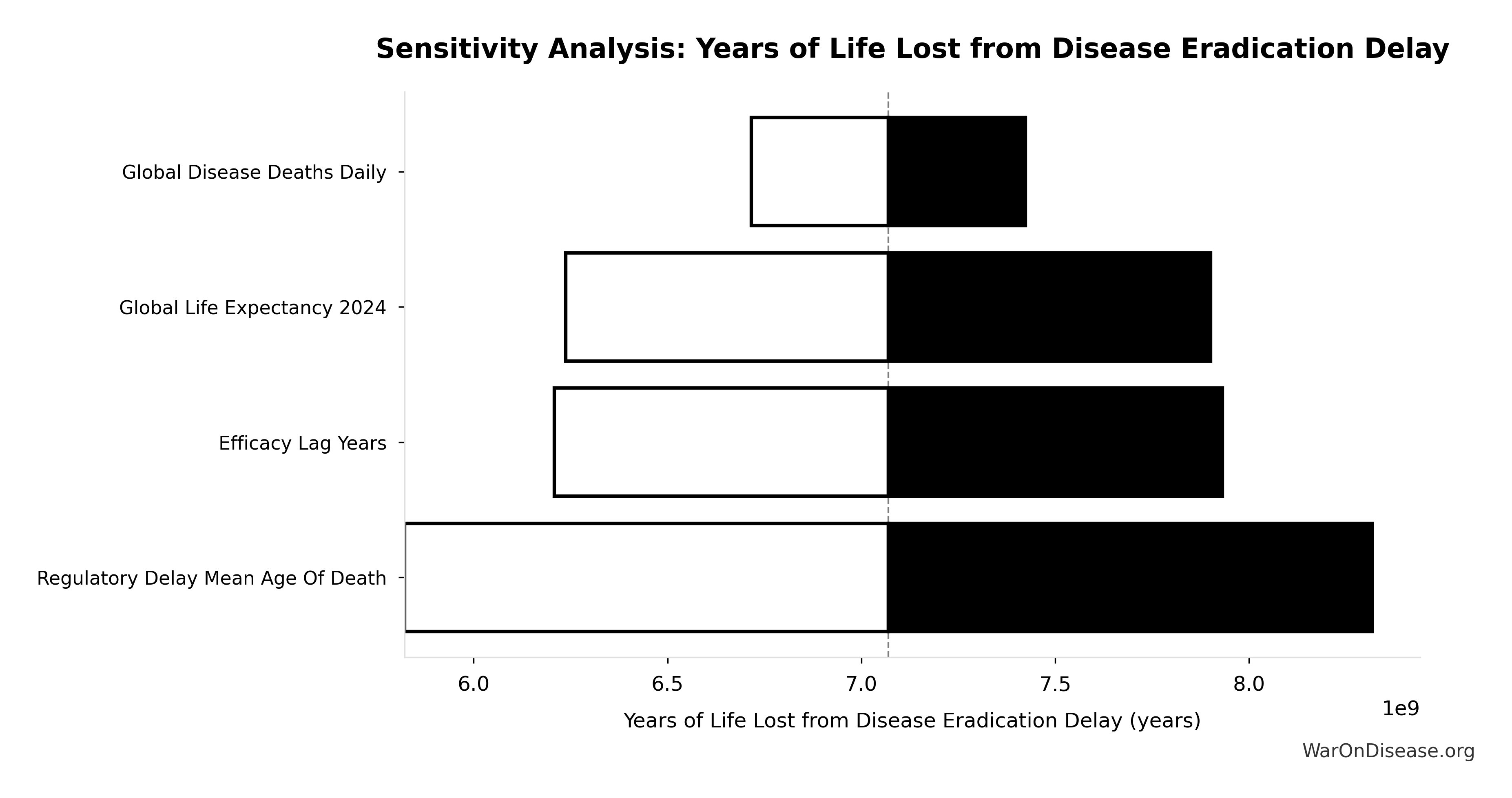
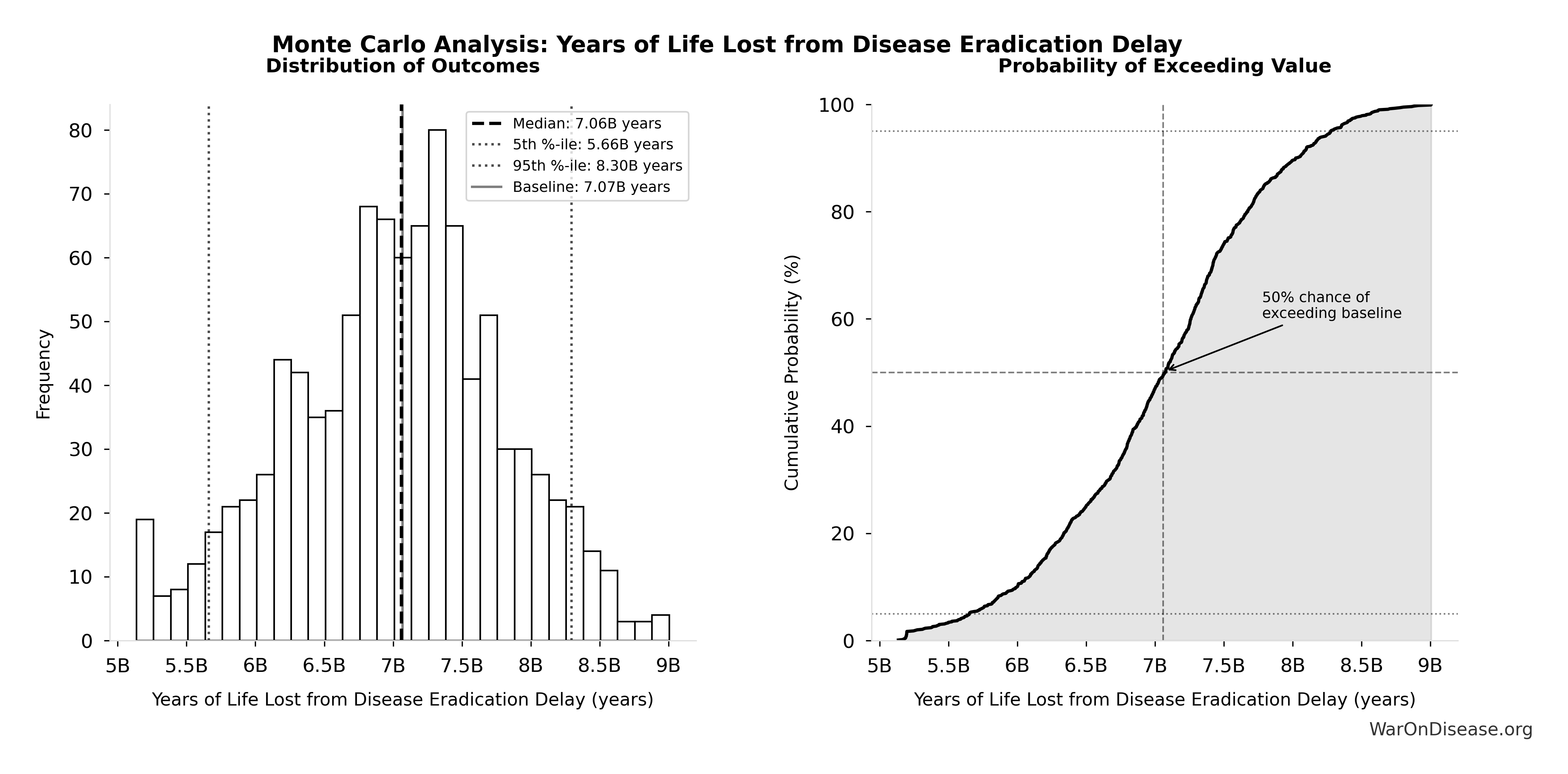
Years of Life Lost from Disease Eradication Delay: 7.07 billion years
Note📊 Details
Years of Life Lost from disease eradication delay deaths (PRIMARY estimate)
Inputs:
- Total Deaths from Disease Eradication Delay 🔢: 416 million deaths
- Global Life Expectancy (2024) 📊: 79 years (SE: ±2 years)
- Mean Age of Preventable Death from Post-Safety Efficacy Delay 📊: 62 years (SE: ±3 years)
\[ \begin{gathered} YLL_{lag} \\ = Deaths_{lag} \times (LE_{global} - Age_{death,delay}) \\ = 416M \times (79 - 62) \\ = 7.07B \end{gathered} \] where: \[ \begin{gathered} Deaths_{lag} \\ = T_{lag} \times Deaths_{disease,daily} \times 338 \\ = 8.2 \times 150{,}000 \times 338 \\ = 416M \end{gathered} \] ~ Medium confidence
Sensitivity Analysis
Sensitivity Indices for Years of Life Lost from Disease Eradication Delay
Regression-based sensitivity showing which inputs explain the most variance in the output.
| Input Parameter | Sensitivity Coefficient | Interpretation |
|---|---|---|
| Global Life Expectancy (2024) (years) | 2.0066 | Strong driver |
| Mean Age of Preventable Death from Post-Safety Efficacy Delay (years) | -1.3852 | Strong driver |
| Total Deaths from Disease Eradication Delay (deaths) | 0.3779 | Moderate driver |
Interpretation: Standardized coefficients show the change in output (in SD units) per 1 SD change in input. Values near ±1 indicate strong influence; values exceeding ±1 may occur with correlated inputs.
Monte Carlo Distribution

Simulation Results Summary: Years of Life Lost from Disease Eradication Delay
| Statistic | Value |
|---|---|
| Baseline (deterministic) | 7.07 billion |
| Mean (expected value) | 7.03 billion |
| Median (50th percentile) | 7.05 billion |
| Standard Deviation | 1.62 billion |
| 90% Range (5th-95th percentile) | [4.21 billion, 9.68 billion] |
The histogram shows the distribution of Years of Life Lost from Disease Eradication Delay across 10,000 Monte Carlo simulations. The CDF (right) shows the probability of the outcome exceeding any given value, which is useful for risk assessment.
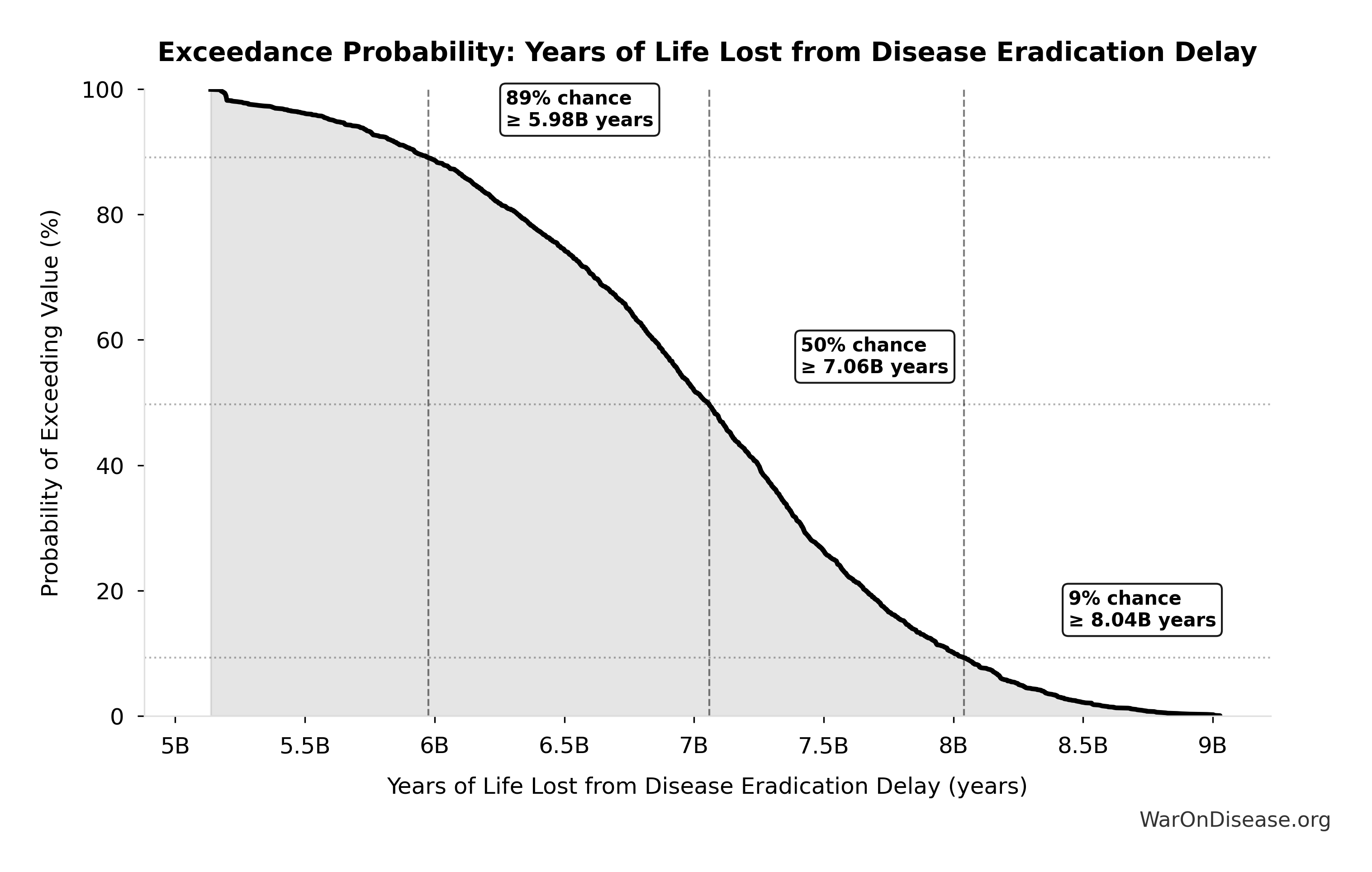
Exceedance Probability
This exceedance probability chart shows the likelihood that Years of Life Lost from Disease Eradication Delay will exceed any given threshold. Higher curves indicate more favorable outcomes with greater certainty.
dFDA New Treatments Per Year: 185 diseases/year
Note📊 Details
Diseases per year receiving their first effective treatment with dFDA. Scales proportionally with trial capacity multiplier.
Inputs:
- Diseases Getting First Treatment Per Year 📊: 15 diseases/year (95% CI: 8 diseases/year - 30 diseases/year)
- Trial Capacity Multiplier 🔢: 12.3x
\[ \begin{gathered} Treatments_{dFDA,ann} \\ = Treatments_{new,ann} \times k_{capacity} \\ = 15 \times 12.3 \\ = 185 \end{gathered} \] where: \[ \begin{gathered} k_{capacity} \\ = \frac{N_{fundable,dFDA}}{Slots_{curr}} \\ = \frac{23.4M}{1.9M} \\ = 12.3 \end{gathered} \] where: \[ \begin{gathered} N_{fundable,dFDA} \\ = \frac{Subsidies_{dFDA,ann}}{Cost_{pragmatic,pt}} \\ = \frac{\$21.8B}{\$929} \\ = 23.4M \end{gathered} \] where: \[ \begin{gathered} Subsidies_{dFDA,ann} \\ = Funding_{dFDA,ann} - OPEX_{dFDA} \\ = \$21.8B - \$40M \\ = \$21.8B \end{gathered} \] where: \[ \begin{gathered} OPEX_{dFDA} \\ = Cost_{platform} + Cost_{staff} + Cost_{infra} \\ + Cost_{regulatory} + Cost_{community} \\ = \$15M + \$10M + \$8M + \$5M + \$2M \\ = \$40M \end{gathered} \] ? Low confidence
Sensitivity Analysis
Sensitivity Indices for dFDA New Treatments Per Year
Regression-based sensitivity showing which inputs explain the most variance in the output.
| Input Parameter | Sensitivity Coefficient | Interpretation |
|---|---|---|
| Trial Capacity Multiplier (x) | 0.9380 | Strong driver |
| Diseases Getting First Treatment Per Year (diseases/year) | -0.0784 | Minimal effect |
Interpretation: Standardized coefficients show the change in output (in SD units) per 1 SD change in input. Values near ±1 indicate strong influence; values exceeding ±1 may occur with correlated inputs.
Monte Carlo Distribution
Simulation Results Summary: dFDA New Treatments Per Year
| Statistic | Value |
|---|---|
| Baseline (deterministic) | 185 |
| Mean (expected value) | 254 |
| Median (50th percentile) | 224 |
| Standard Deviation | 141 |
| 90% Range (5th-95th percentile) | [107, 491] |
The histogram shows the distribution of dFDA New Treatments Per Year across 10,000 Monte Carlo simulations. The CDF (right) shows the probability of the outcome exceeding any given value, which is useful for risk assessment.
Exceedance Probability
This exceedance probability chart shows the likelihood that dFDA New Treatments Per Year will exceed any given threshold. Higher curves indicate more favorable outcomes with greater certainty.
Maximum Trial Capacity Multiplier (Physical Limit): 566x
Note📊 Details
Physical upper bound on trial-capacity multiplier from participant availability. Even with unlimited funding, annual trial enrollment cannot exceed willing participant pool.
Inputs:
- Global Patients Willing to Participate in Clinical Trials 🔢: 1.08 billion people
- Annual Global Clinical Trial Participants 📊: 1.9 million patients/year (95% CI: 1.5 million patients/year - 2.3 million patients/year)
\[ \begin{gathered} k_{capacity,max} \\ = \frac{N_{willing}}{Slots_{curr}} \\ = \frac{1.08B}{1.9M} \\ = 566 \end{gathered} \] where: \[ \begin{gathered} N_{willing} \\ = N_{patients} \times Pct_{willing} \\ = 2.4B \times 44.8\% \\ = 1.08B \end{gathered} \] ~ Medium confidence
Sensitivity Analysis
Sensitivity Indices for Maximum Trial Capacity Multiplier (Physical Limit)
Regression-based sensitivity showing which inputs explain the most variance in the output.
| Input Parameter | Sensitivity Coefficient | Interpretation |
|---|---|---|
| Global Patients Willing to Participate in Clinical Trials (people) | 0.8980 | Strong driver |
| Annual Global Clinical Trial Participants (patients/year) | 0.0989 | Minimal effect |
Interpretation: Standardized coefficients show the change in output (in SD units) per 1 SD change in input. Values near ±1 indicate strong influence; values exceeding ±1 may occur with correlated inputs.
Monte Carlo Distribution
Simulation Results Summary: Maximum Trial Capacity Multiplier (Physical Limit)
| Statistic | Value |
|---|---|
| Baseline (deterministic) | 566x |
| Mean (expected value) | 567x |
| Median (50th percentile) | 567x |
| Standard Deviation | 18.4x |
| 90% Range (5th-95th percentile) | [534x, 597x] |
The histogram shows the distribution of Maximum Trial Capacity Multiplier (Physical Limit) across 10,000 Monte Carlo simulations. The CDF (right) shows the probability of the outcome exceeding any given value, which is useful for risk assessment.
Exceedance Probability
This exceedance probability chart shows the likelihood that Maximum Trial Capacity Multiplier (Physical Limit) will exceed any given threshold. Higher curves indicate more favorable outcomes with greater certainty.
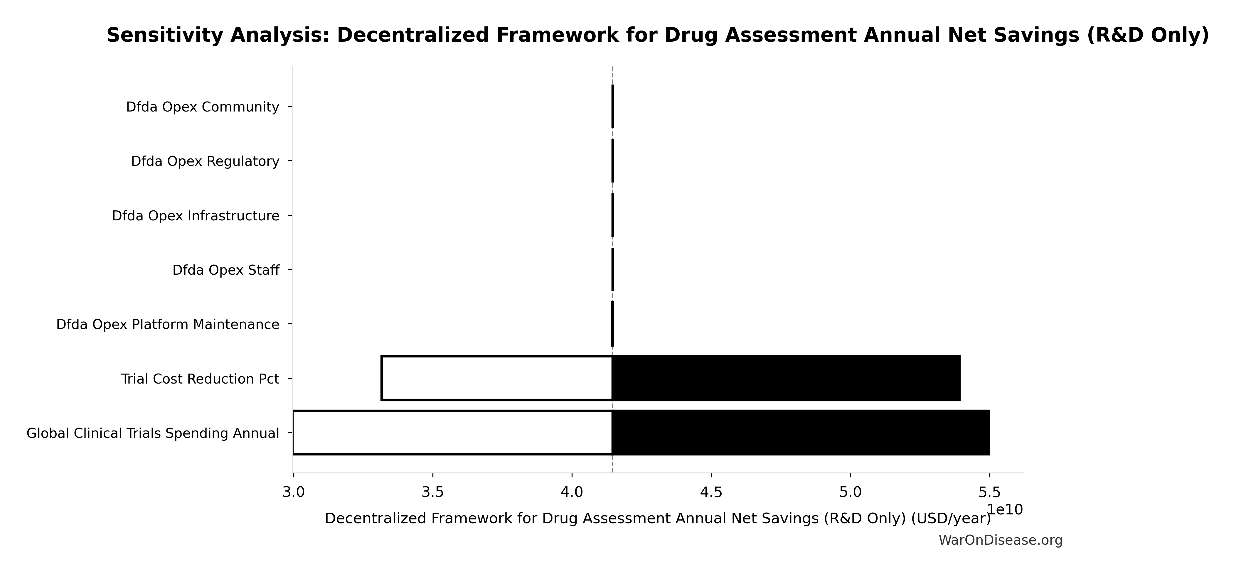
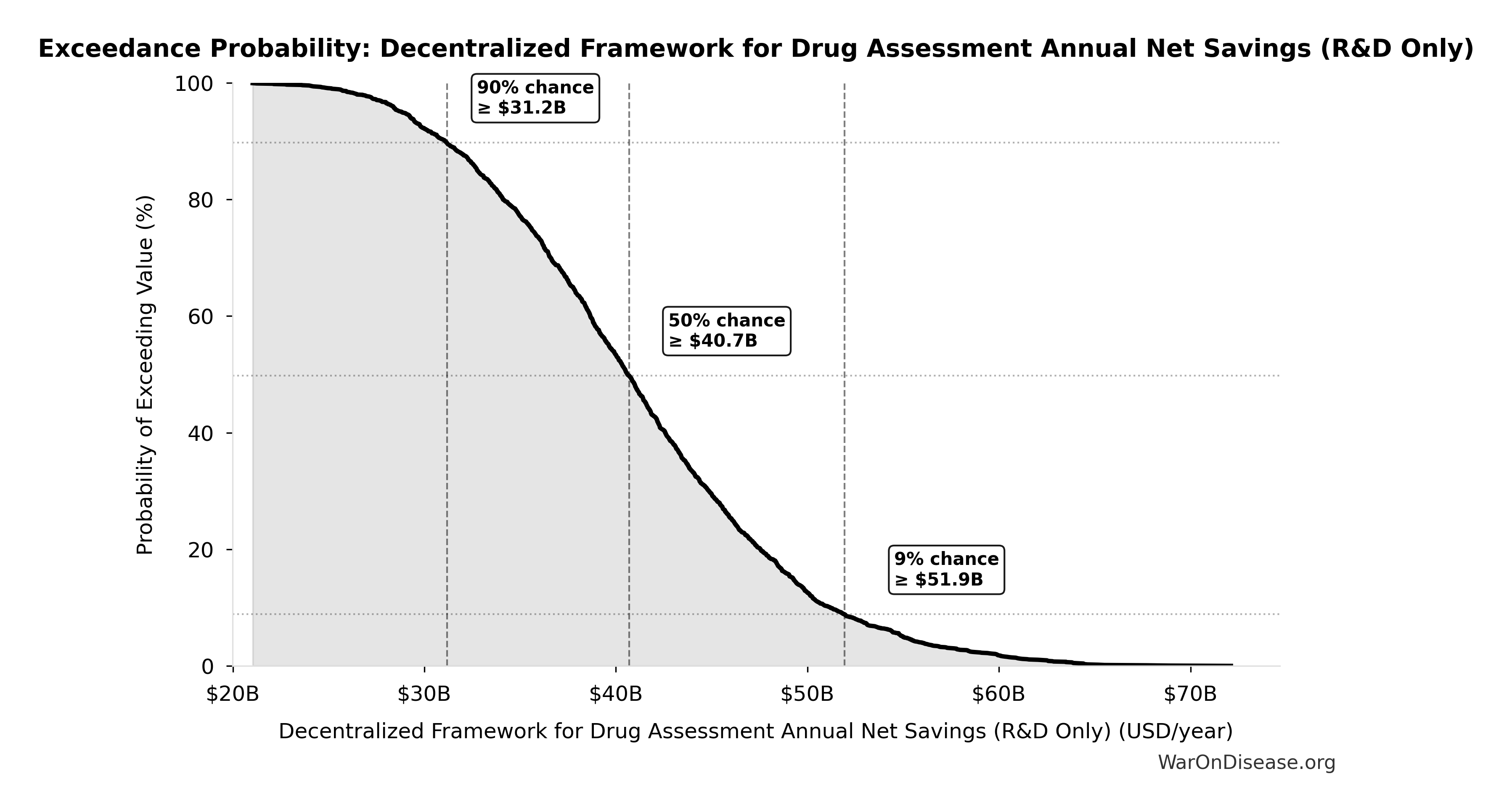
Decentralized Framework for Drug Assessment Annual Net Savings (R&D Only): $58.6B
Note📊 Details
Annual net savings from R&D cost reduction only (gross savings minus operational costs, excludes regulatory delay value)
Inputs:
- Decentralized Framework for Drug Assessment Annual Benefit: R&D Savings 🔢: $58.6B
- Total Annual Decentralized Framework for Drug Assessment Operational Costs 🔢: $40M
\[ \begin{gathered} Savings_{RD,ann} \\ = Benefit_{RD,ann} - OPEX_{dFDA} \\ = \$58.6B - \$40M \\ = \$58.6B \end{gathered} \] where: \[ \begin{gathered} Benefit_{RD,ann} \\ = Spending_{trials} \times Reduce_{pct} \\ = \$60B \times 97.7\% \\ = \$58.6B \end{gathered} \] where: \[ \begin{gathered} Reduce_{pct} \\ = 1 - \frac{Cost_{pragmatic,pt}}{Cost_{P3,pt}} \\ = 1 - \frac{\$929}{\$41K} \\ = 97.7\% \end{gathered} \] where: \[ \begin{gathered} OPEX_{dFDA} \\ = Cost_{platform} + Cost_{staff} + Cost_{infra} \\ + Cost_{regulatory} + Cost_{community} \\ = \$15M + \$10M + \$8M + \$5M + \$2M \\ = \$40M \end{gathered} \] ✓ High confidence
Sensitivity Analysis

Sensitivity Indices for Decentralized Framework for Drug Assessment Annual Net Savings (R&D Only)
Regression-based sensitivity showing which inputs explain the most variance in the output.
| Input Parameter | Sensitivity Coefficient | Interpretation |
|---|---|---|
| Decentralized Framework for Drug Assessment Annual Benefit: R&D Savings (USD/year) | 1.0011 | Strong driver |
| Total Annual Decentralized Framework for Drug Assessment Operational Costs (USD/year) | -0.0011 | Minimal effect |
Interpretation: Standardized coefficients show the change in output (in SD units) per 1 SD change in input. Values near ±1 indicate strong influence; values exceeding ±1 may occur with correlated inputs.
Monte Carlo Distribution
Simulation Results Summary: Decentralized Framework for Drug Assessment Annual Net Savings (R&D Only)
| Statistic | Value |
|---|---|
| Baseline (deterministic) | $58.6B |
| Mean (expected value) | $58.8B |
| Median (50th percentile) | $57.8B |
| Standard Deviation | $7.66B |
| 90% Range (5th-95th percentile) | [$49.2B, $73B] |
The histogram shows the distribution of Decentralized Framework for Drug Assessment Annual Net Savings (R&D Only) across 10,000 Monte Carlo simulations. The CDF (right) shows the probability of the outcome exceeding any given value, which is useful for risk assessment.
Exceedance Probability
This exceedance probability chart shows the likelihood that Decentralized Framework for Drug Assessment Annual Net Savings (R&D Only) will exceed any given threshold. Higher curves indicate more favorable outcomes with greater certainty.
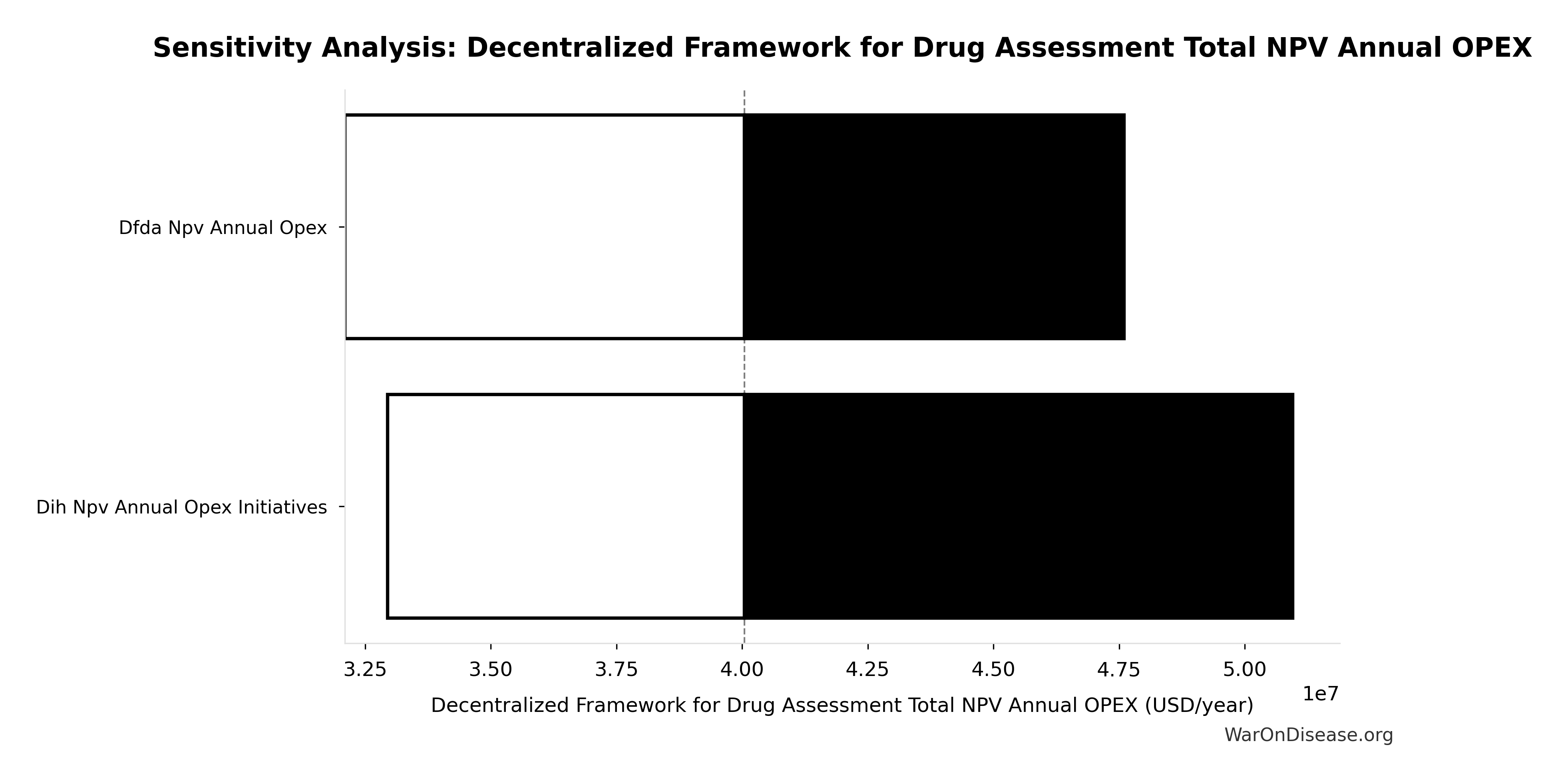
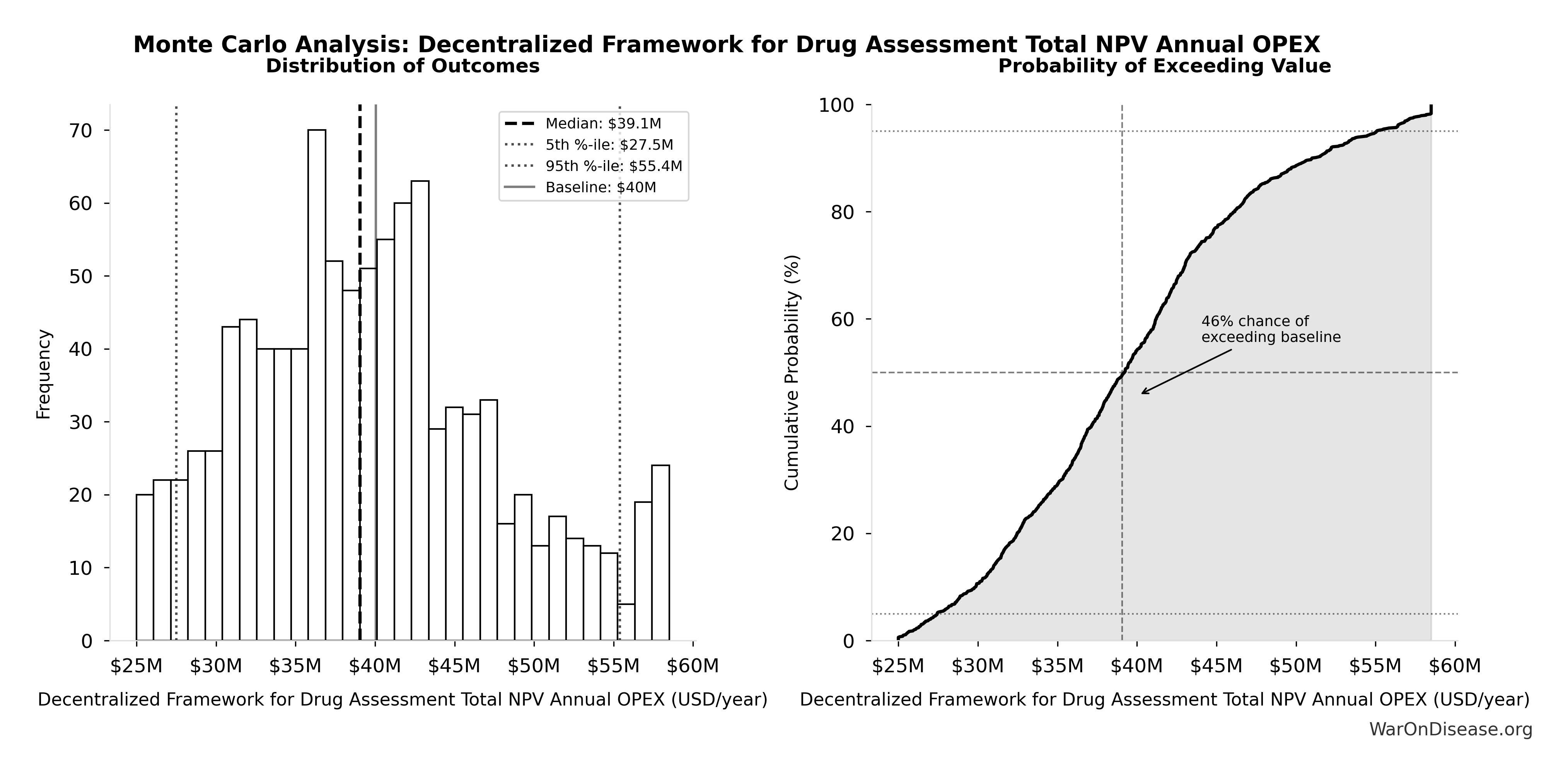
Decentralized Framework for Drug Assessment Total NPV Annual OPEX: $40M
Note📊 Details
Total NPV annual opex (Decentralized Framework for Drug Assessment core + DIH initiatives)
Inputs:
- Decentralized Framework for Drug Assessment Core framework Annual OPEX: $18.9M (95% CI: $11M - $26.5M)
- DIH Broader Initiatives Annual OPEX: $21.1M (95% CI: $14M - $32M)
\[ \begin{gathered} OPEX_{total} \\ = OPEX_{ann} + OPEX_{DIH,ann} \\ = \$18.9M + \$21.1M \\ = \$40M \end{gathered} \]
✓ High confidence
Sensitivity Analysis
Sensitivity Indices for Decentralized Framework for Drug Assessment Total NPV Annual OPEX
Regression-based sensitivity showing which inputs explain the most variance in the output.
| Input Parameter | Sensitivity Coefficient | Interpretation |
|---|---|---|
| DIH Broader Initiatives Annual OPEX (USD/year) | 0.5419 | Strong driver |
| Decentralized Framework for Drug Assessment Core framework Annual OPEX (USD/year) | 0.4592 | Moderate driver |
Interpretation: Standardized coefficients show the change in output (in SD units) per 1 SD change in input. Values near ±1 indicate strong influence; values exceeding ±1 may occur with correlated inputs.
Monte Carlo Distribution
Simulation Results Summary: Decentralized Framework for Drug Assessment Total NPV Annual OPEX
| Statistic | Value |
|---|---|
| Baseline (deterministic) | $40M |
| Mean (expected value) | $39.9M |
| Median (50th percentile) | $39.1M |
| Standard Deviation | $8.04M |
| 90% Range (5th-95th percentile) | [$27.5M, $55.4M] |
The histogram shows the distribution of Decentralized Framework for Drug Assessment Total NPV Annual OPEX across 10,000 Monte Carlo simulations. The CDF (right) shows the probability of the outcome exceeding any given value, which is useful for risk assessment.
Exceedance Probability
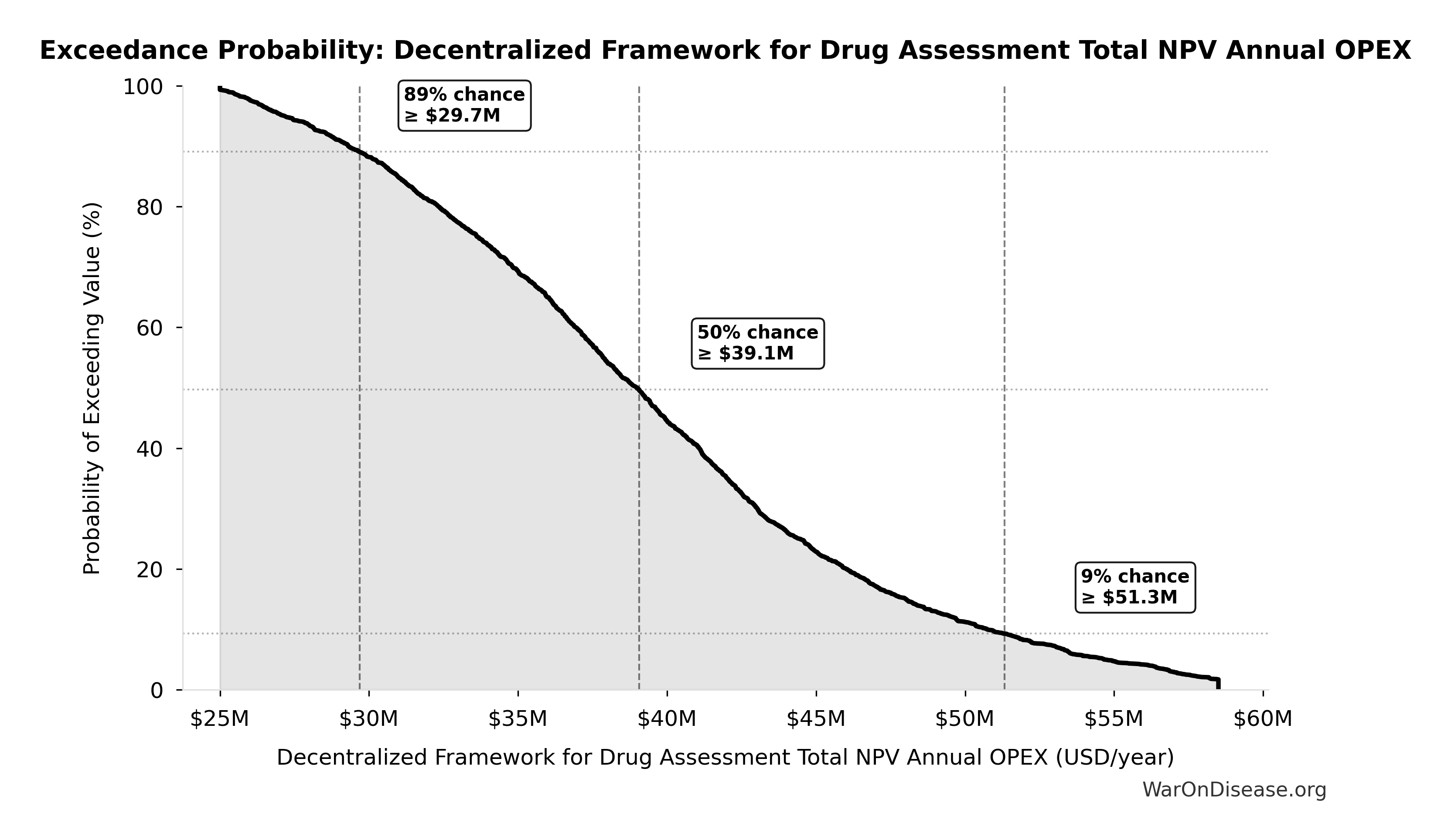
This exceedance probability chart shows the likelihood that Decentralized Framework for Drug Assessment Total NPV Annual OPEX will exceed any given threshold. Higher curves indicate more favorable outcomes with greater certainty.
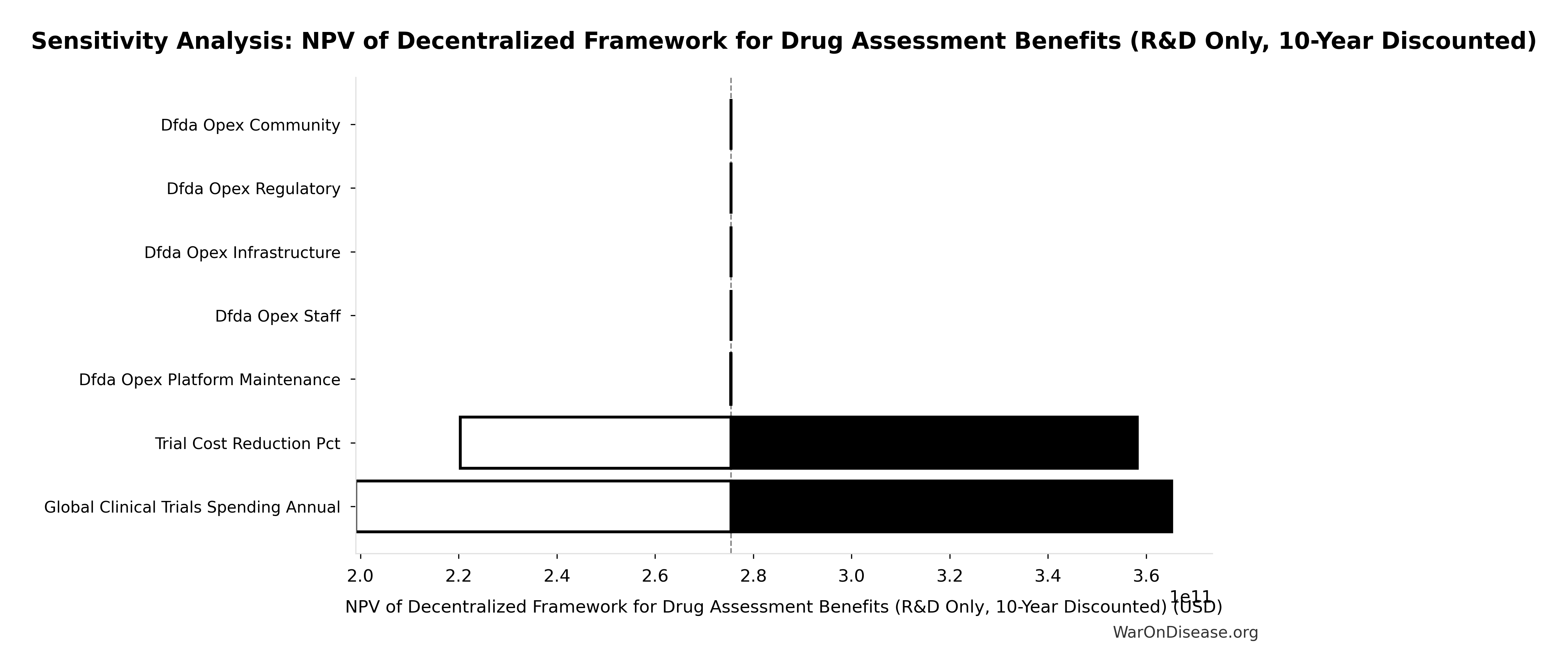
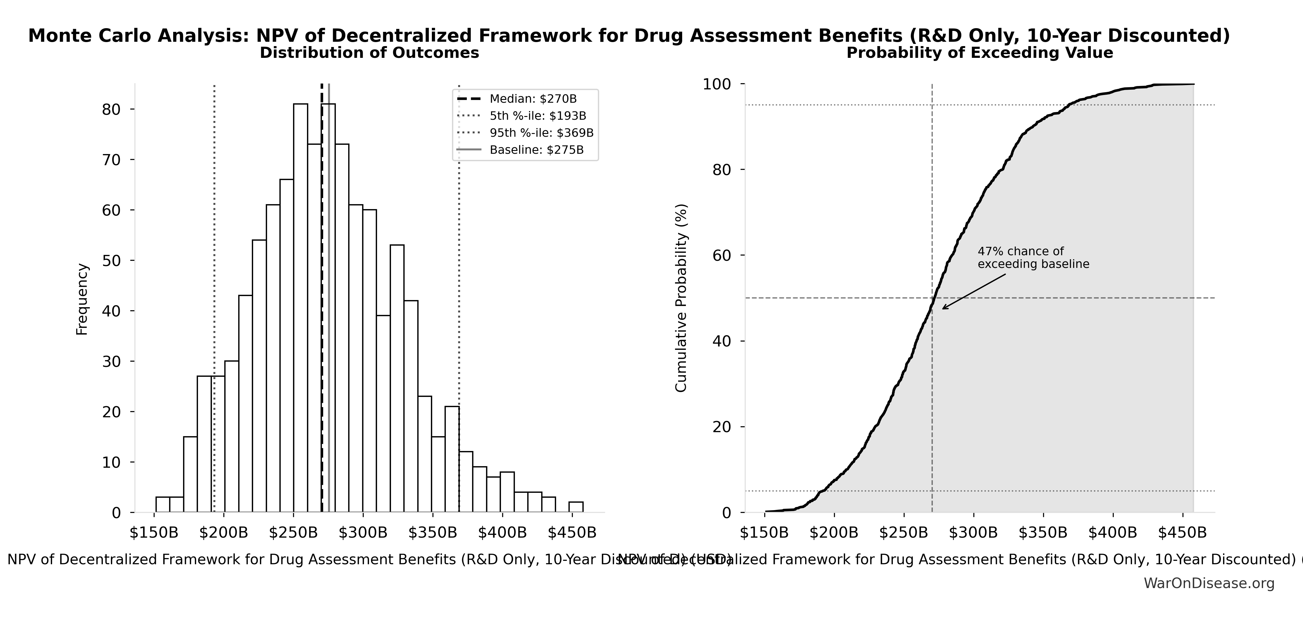
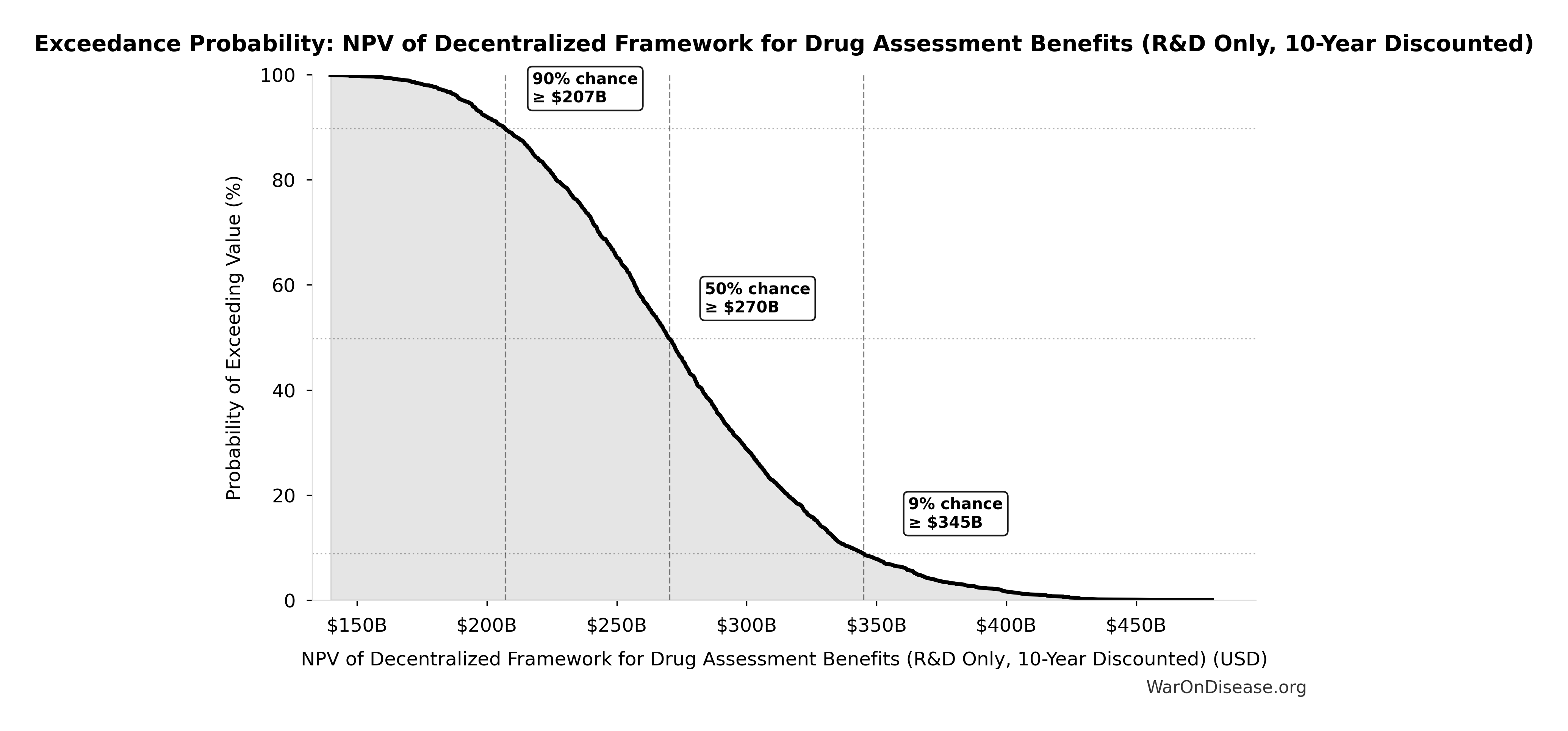
NPV of Decentralized Framework for Drug Assessment Benefits (R&D Only, 10-Year Discounted): $389B
Note📊 Details
NPV of Decentralized Framework for Drug Assessment R&D savings only with 5-year adoption ramp (10-year horizon, most conservative financial estimate)
Inputs:
- Decentralized Framework for Drug Assessment Annual Net Savings (R&D Only) 🔢: $58.6B
- Standard Discount Rate for NPV Analysis: 3%
\[ \begin{gathered} NPV_{RD} \\ = \sum_{t=1}^{10} \frac{Savings_{RD,ann} \times \frac{\min(t,5)}{5}}{(1+r)^t} \end{gathered} \]
✓ High confidence
Sensitivity Analysis
Sensitivity Indices for NPV of Decentralized Framework for Drug Assessment Benefits (R&D Only, 10-Year Discounted)
Regression-based sensitivity showing which inputs explain the most variance in the output.
| Input Parameter | Sensitivity Coefficient | Interpretation |
|---|---|---|
| Decentralized Framework for Drug Assessment Annual Net Savings (R&D Only) (USD/year) | 1.0000 | Strong driver |
Interpretation: Standardized coefficients show the change in output (in SD units) per 1 SD change in input. Values near ±1 indicate strong influence; values exceeding ±1 may occur with correlated inputs.
Monte Carlo Distribution
Simulation Results Summary: NPV of Decentralized Framework for Drug Assessment Benefits (R&D Only, 10-Year Discounted)
| Statistic | Value |
|---|---|
| Baseline (deterministic) | $389B |
| Mean (expected value) | $391B |
| Median (50th percentile) | $384B |
| Standard Deviation | $50.9B |
| 90% Range (5th-95th percentile) | [$327B, $485B] |
The histogram shows the distribution of NPV of Decentralized Framework for Drug Assessment Benefits (R&D Only, 10-Year Discounted) across 10,000 Monte Carlo simulations. The CDF (right) shows the probability of the outcome exceeding any given value, which is useful for risk assessment.
Exceedance Probability
This exceedance probability chart shows the likelihood that NPV of Decentralized Framework for Drug Assessment Benefits (R&D Only, 10-Year Discounted) will exceed any given threshold. Higher curves indicate more favorable outcomes with greater certainty.
NPV Net Benefit (R&D Only): $389B
Note📊 Details
NPV net benefit using R&D savings only (benefits minus costs)
Inputs:
- NPV of Decentralized Framework for Drug Assessment Benefits (R&D Only, 10-Year Discounted) 🔢: $389B
- Decentralized Framework for Drug Assessment Total NPV Cost 🔢: $611M
\[ \begin{gathered} NPV_{net,RD} \\ = NPV_{RD} - Cost_{dFDA,total} \\ = \$389B - \$611M \\ = \$389B \end{gathered} \] where: \[ \begin{gathered} NPV_{RD} \\ = \sum_{t=1}^{10} \frac{Savings_{RD,ann} \times \frac{\min(t,5)}{5}}{(1+r)^t} \end{gathered} \] where: \[ \begin{gathered} Savings_{RD,ann} \\ = Benefit_{RD,ann} - OPEX_{dFDA} \\ = \$58.6B - \$40M \\ = \$58.6B \end{gathered} \] where: \[ \begin{gathered} Benefit_{RD,ann} \\ = Spending_{trials} \times Reduce_{pct} \\ = \$60B \times 97.7\% \\ = \$58.6B \end{gathered} \] where: \[ \begin{gathered} Reduce_{pct} \\ = 1 - \frac{Cost_{pragmatic,pt}}{Cost_{P3,pt}} \\ = 1 - \frac{\$929}{\$41K} \\ = 97.7\% \end{gathered} \] where: \[ \begin{gathered} OPEX_{dFDA} \\ = Cost_{platform} + Cost_{staff} + Cost_{infra} \\ + Cost_{regulatory} + Cost_{community} \\ = \$15M + \$10M + \$8M + \$5M + \$2M \\ = \$40M \end{gathered} \] where: \[ \begin{gathered} Cost_{dFDA,total} \\ = PV_{OPEX} + Cost_{upfront,total} \\ = \$342M + \$270M \\ = \$611M \end{gathered} \] where: \[ PV_{OPEX} = OPEX_{ann} \times \frac{1 - (1+r)^{-T}}{r} \] where: \[ \begin{gathered} OPEX_{total} \\ = OPEX_{ann} + OPEX_{DIH,ann} \\ = \$18.9M + \$21.1M \\ = \$40M \end{gathered} \] where: \[ \begin{gathered} Cost_{upfront,total} \\ = Cost_{upfront} + Cost_{DIH,init} \\ = \$40M + \$230M \\ = \$270M \end{gathered} \] ✓ High confidence
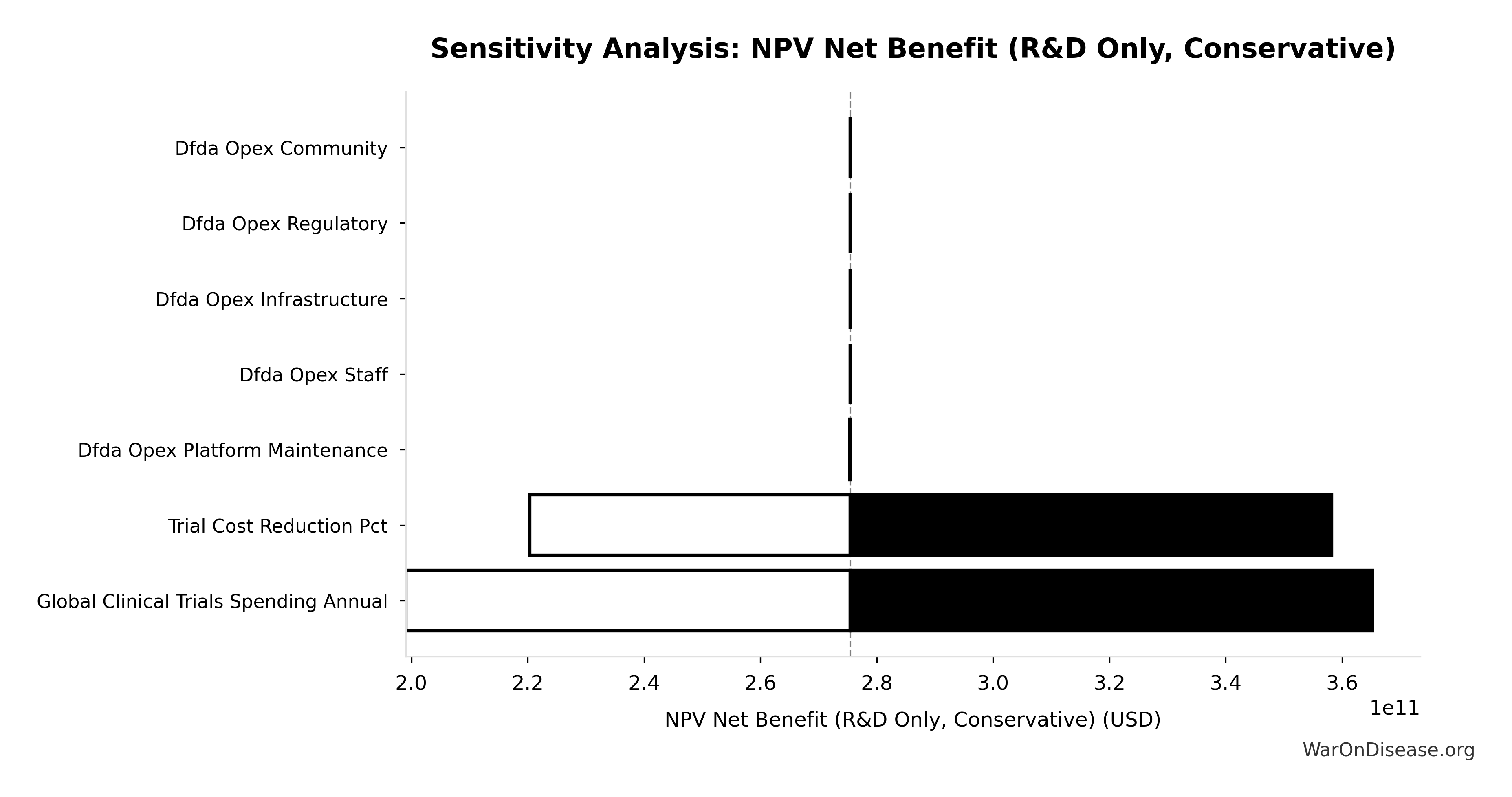
Sensitivity Analysis
Sensitivity Indices for NPV Net Benefit (R&D Only)
Regression-based sensitivity showing which inputs explain the most variance in the output.
| Input Parameter | Sensitivity Coefficient | Interpretation |
|---|---|---|
| NPV of Decentralized Framework for Drug Assessment Benefits (R&D Only, 10-Year Discounted) (USD) | 1.0025 | Strong driver |
| Decentralized Framework for Drug Assessment Total NPV Cost (USD) | -0.0025 | Minimal effect |
Interpretation: Standardized coefficients show the change in output (in SD units) per 1 SD change in input. Values near ±1 indicate strong influence; values exceeding ±1 may occur with correlated inputs.
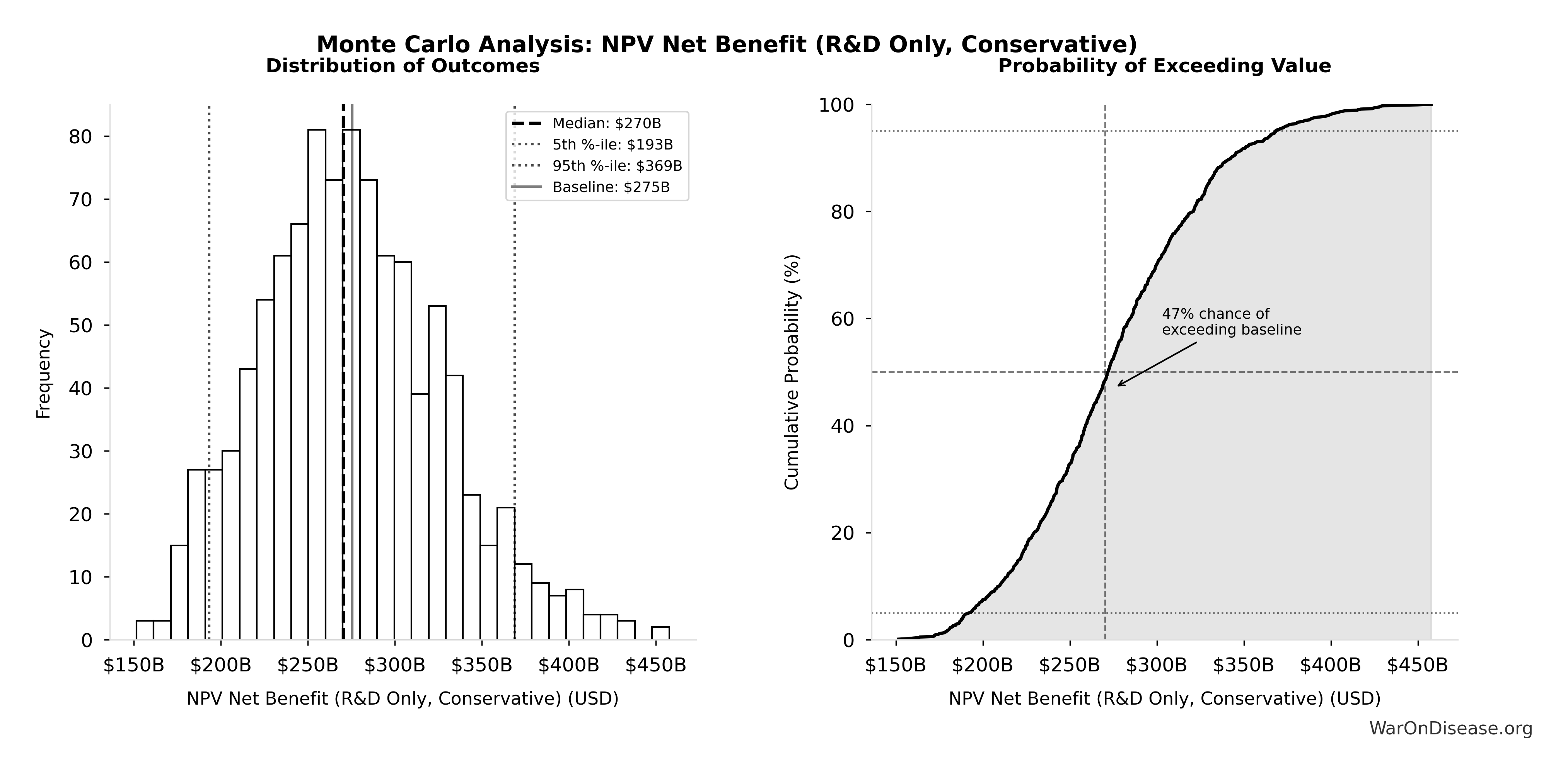
Monte Carlo Distribution
Simulation Results Summary: NPV Net Benefit (R&D Only)
| Statistic | Value |
|---|---|
| Baseline (deterministic) | $389B |
| Mean (expected value) | $390B |
| Median (50th percentile) | $383B |
| Standard Deviation | $50.7B |
| 90% Range (5th-95th percentile) | [$326B, $484B] |
The histogram shows the distribution of NPV Net Benefit (R&D Only) across 10,000 Monte Carlo simulations. The CDF (right) shows the probability of the outcome exceeding any given value, which is useful for risk assessment.
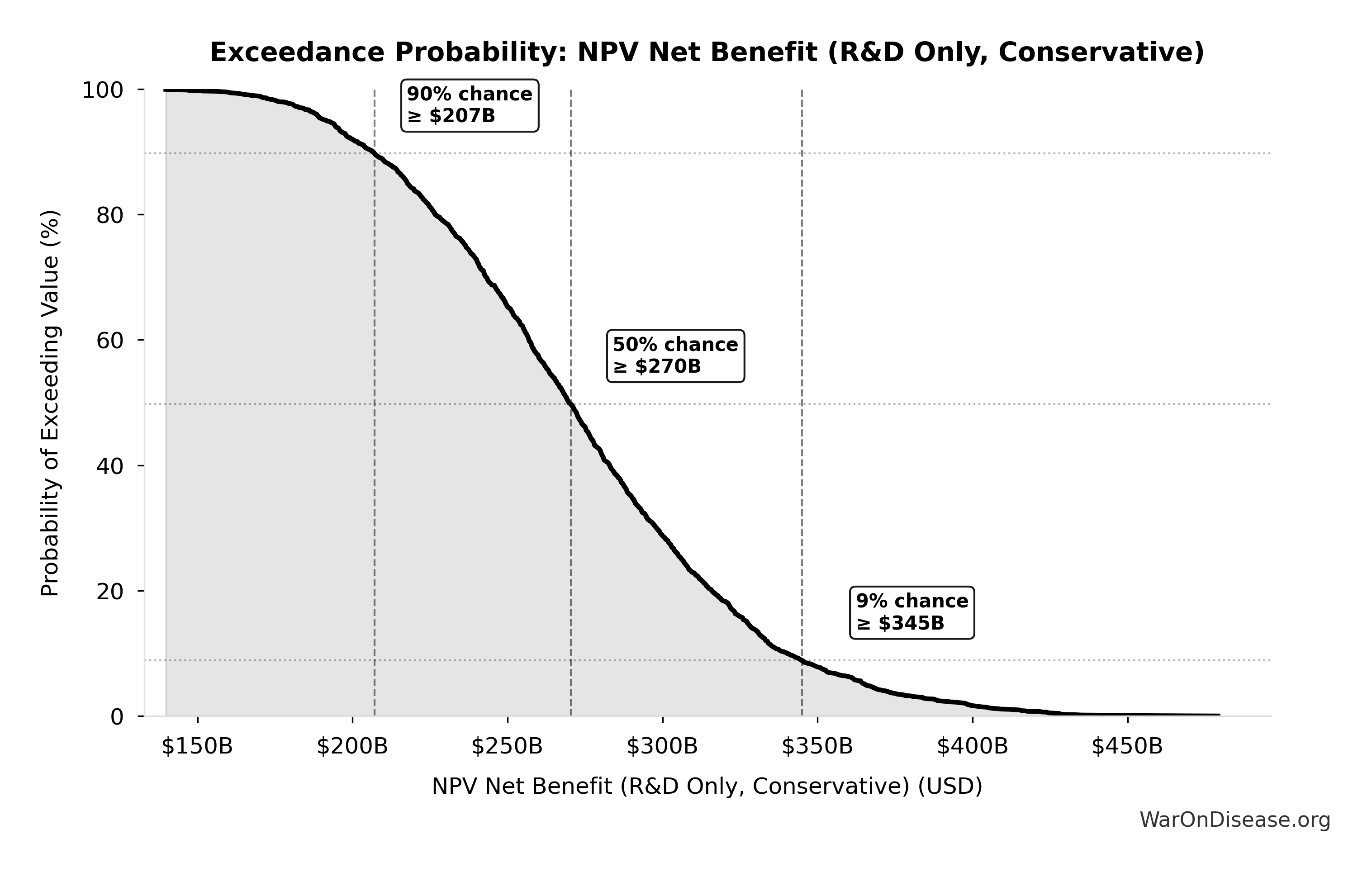
Exceedance Probability
This exceedance probability chart shows the likelihood that NPV Net Benefit (R&D Only) will exceed any given threshold. Higher curves indicate more favorable outcomes with greater certainty.
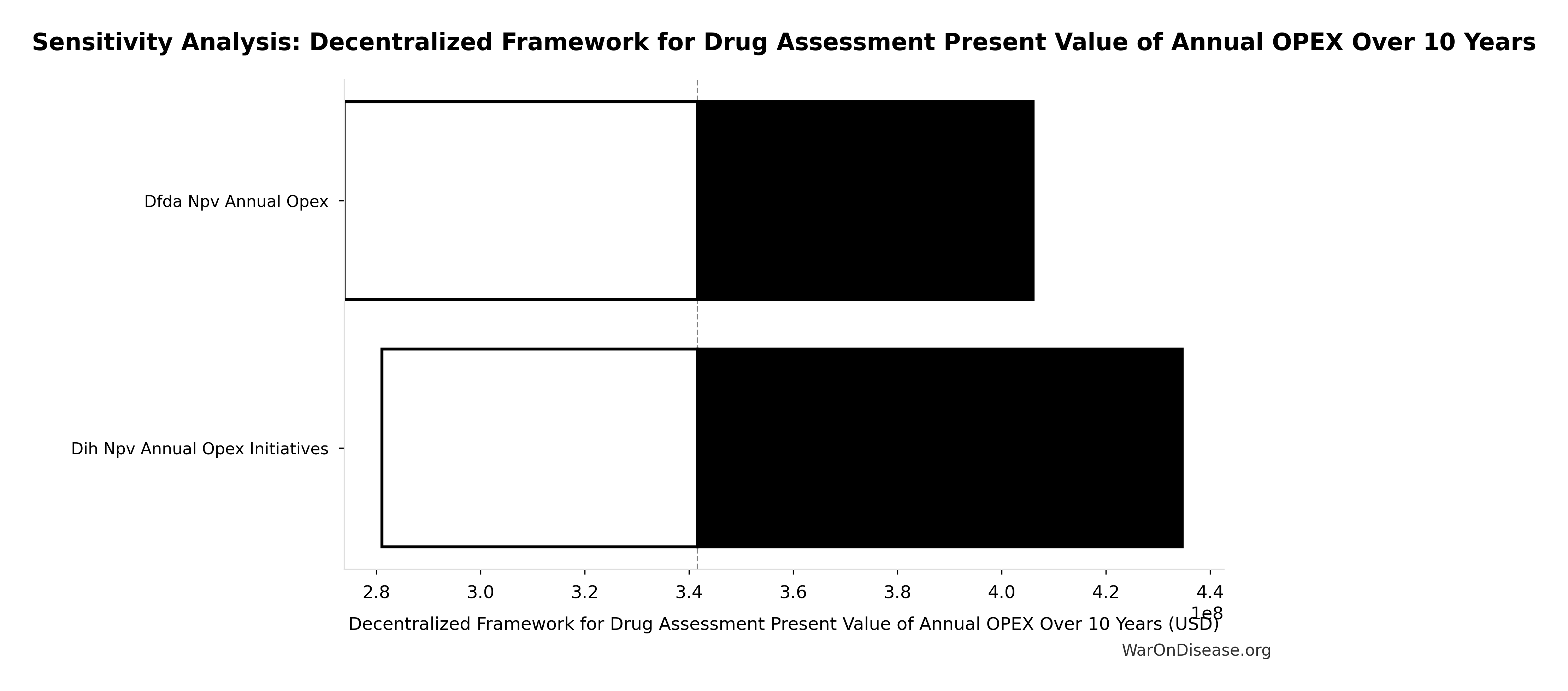
Decentralized Framework for Drug Assessment Present Value of Annual OPEX Over 10 Years: $342M
Note📊 Details
Present value of annual opex over 10 years (NPV formula)
Inputs:
- Decentralized Framework for Drug Assessment Total NPV Annual OPEX 🔢: $40M
- Standard Discount Rate for NPV Analysis: 3%
- Standard Time Horizon for NPV Analysis: 10 years
\[ PV_{OPEX} = OPEX_{ann} \times \frac{1 - (1+r)^{-T}}{r} \]
✓ High confidence
Sensitivity Analysis
Sensitivity Indices for Decentralized Framework for Drug Assessment Present Value of Annual OPEX Over 10 Years
Regression-based sensitivity showing which inputs explain the most variance in the output.
| Input Parameter | Sensitivity Coefficient | Interpretation |
|---|---|---|
| Decentralized Framework for Drug Assessment Total NPV Annual OPEX (USD/year) | 1.0000 | Strong driver |
Interpretation: Standardized coefficients show the change in output (in SD units) per 1 SD change in input. Values near ±1 indicate strong influence; values exceeding ±1 may occur with correlated inputs.
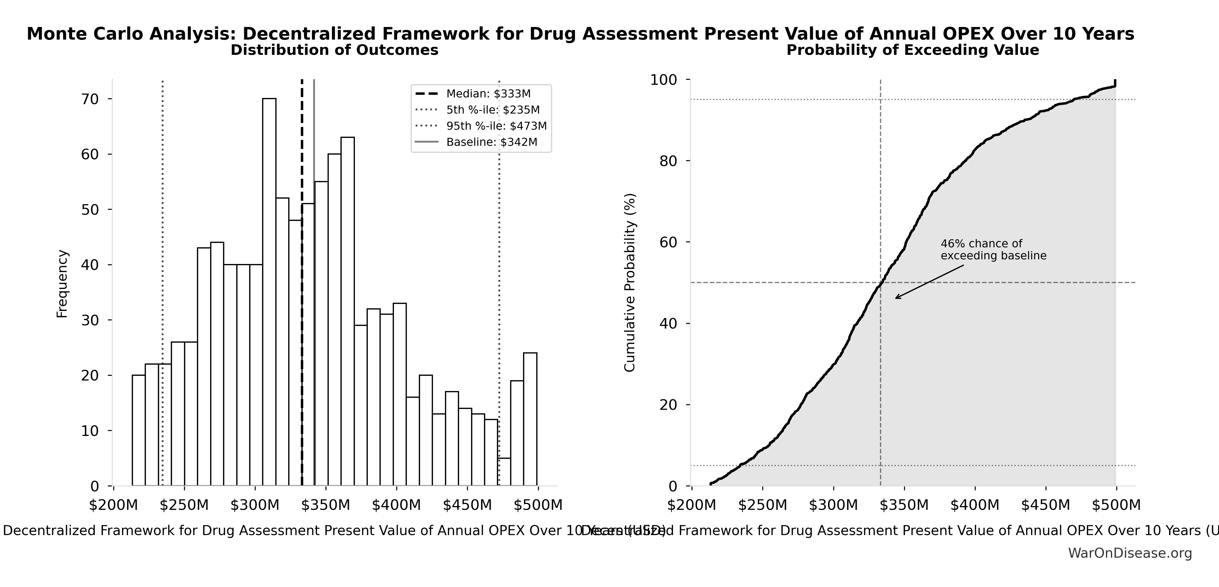
Monte Carlo Distribution
Simulation Results Summary: Decentralized Framework for Drug Assessment Present Value of Annual OPEX Over 10 Years
| Statistic | Value |
|---|---|
| Baseline (deterministic) | $342M |
| Mean (expected value) | $340M |
| Median (50th percentile) | $333M |
| Standard Deviation | $68.6M |
| 90% Range (5th-95th percentile) | [$235M, $473M] |
The histogram shows the distribution of Decentralized Framework for Drug Assessment Present Value of Annual OPEX Over 10 Years across 10,000 Monte Carlo simulations. The CDF (right) shows the probability of the outcome exceeding any given value, which is useful for risk assessment.
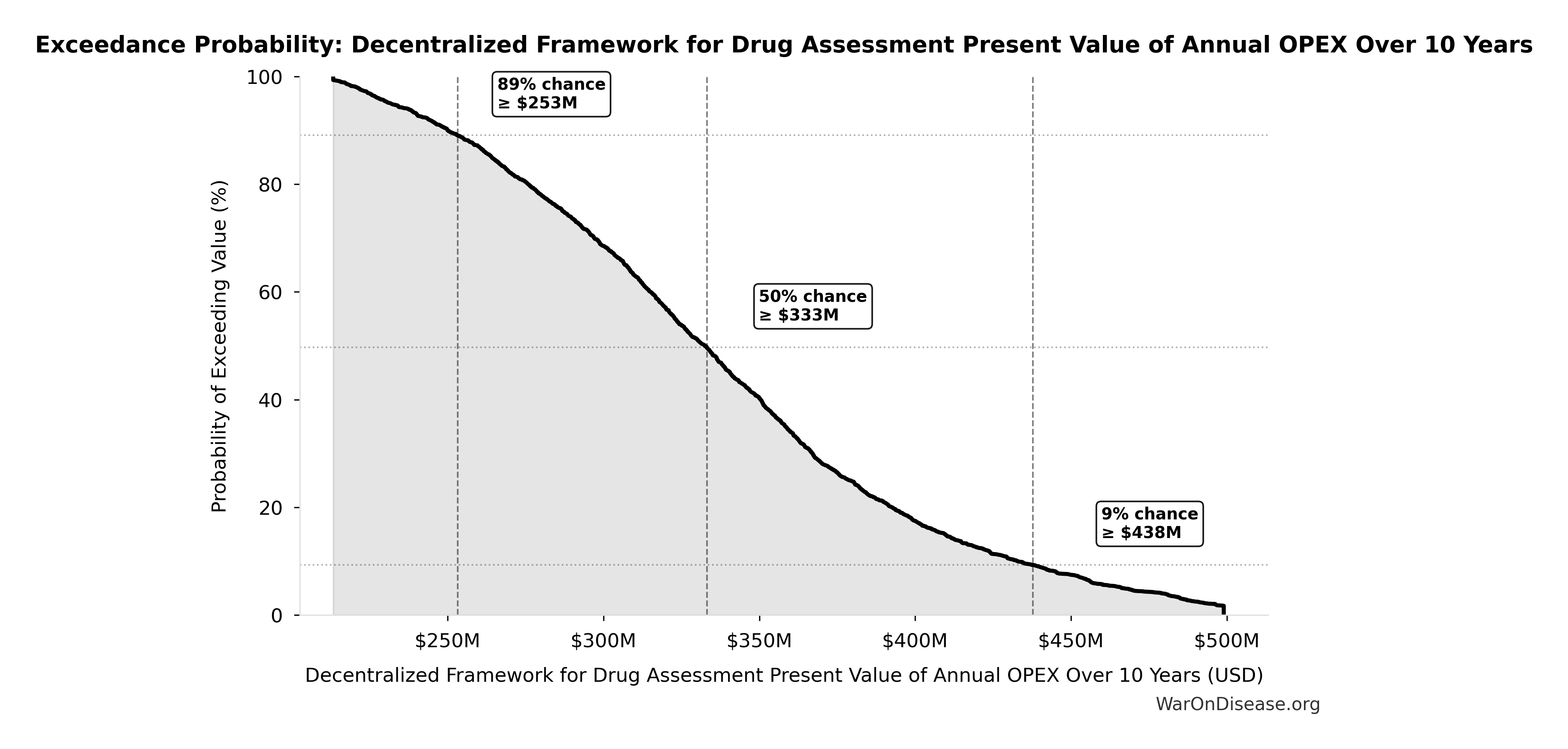
Exceedance Probability
This exceedance probability chart shows the likelihood that Decentralized Framework for Drug Assessment Present Value of Annual OPEX Over 10 Years will exceed any given threshold. Higher curves indicate more favorable outcomes with greater certainty.
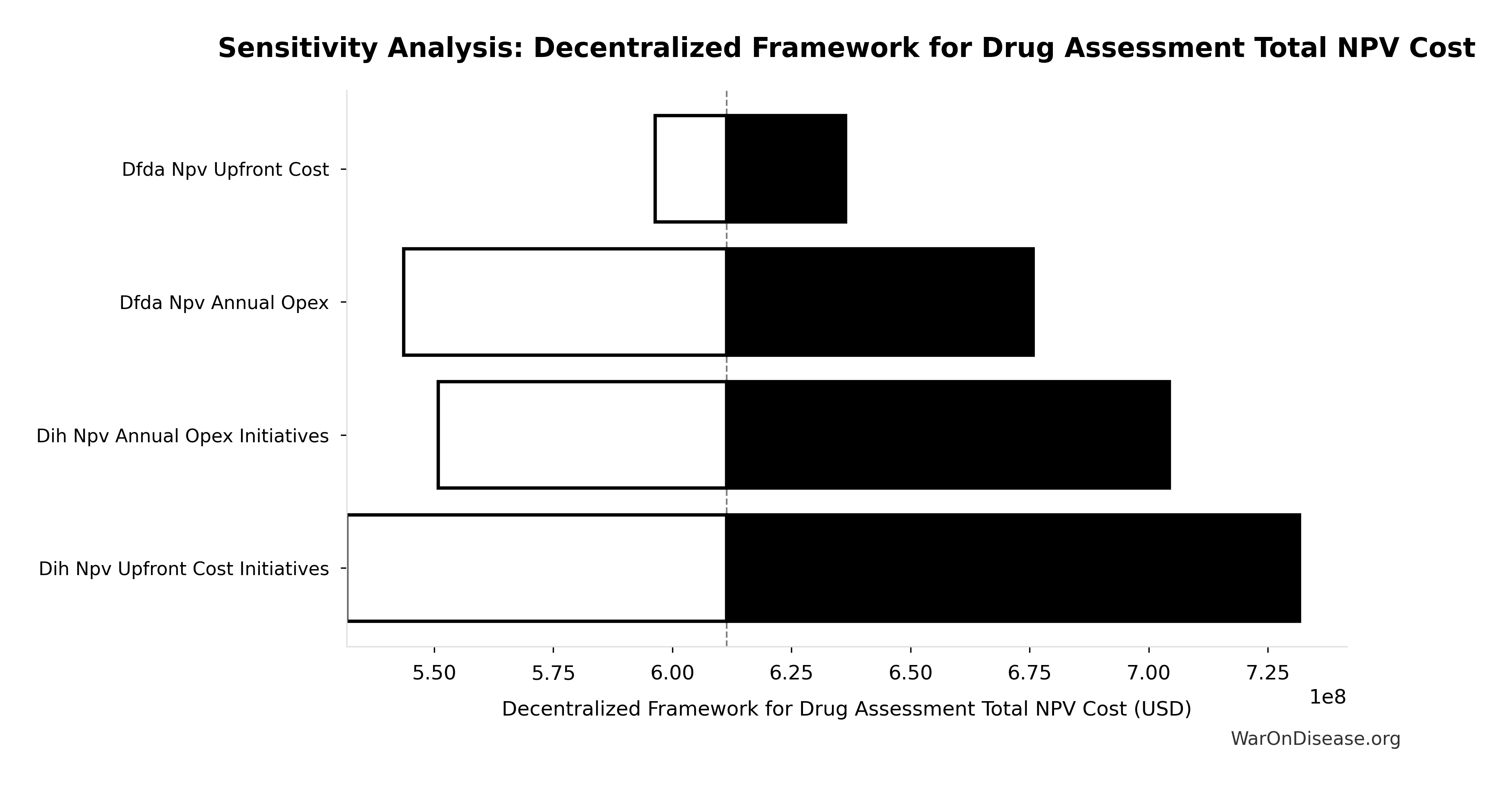
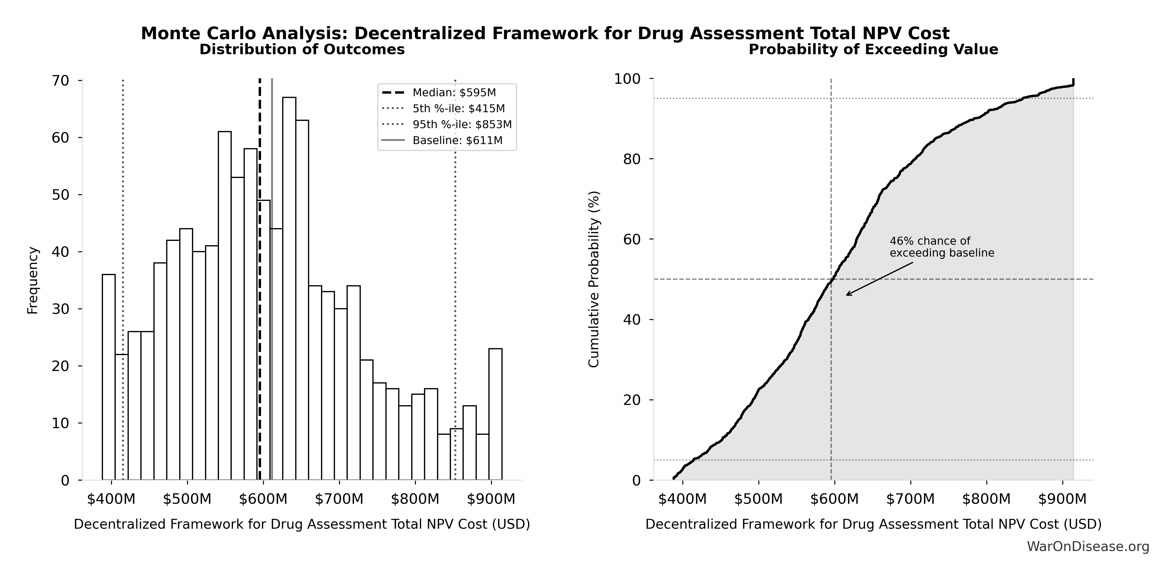
Decentralized Framework for Drug Assessment Total NPV Cost: $611M
Note📊 Details
Total NPV cost (upfront + PV of annual opex)
Inputs:
- Decentralized Framework for Drug Assessment Present Value of Annual OPEX Over 10 Years 🔢: $342M
- Decentralized Framework for Drug Assessment Total NPV Upfront Costs 🔢: $270M
\[ \begin{gathered} Cost_{dFDA,total} \\ = PV_{OPEX} + Cost_{upfront,total} \\ = \$342M + \$270M \\ = \$611M \end{gathered} \] where: \[ PV_{OPEX} = OPEX_{ann} \times \frac{1 - (1+r)^{-T}}{r} \] where: \[ \begin{gathered} OPEX_{total} \\ = OPEX_{ann} + OPEX_{DIH,ann} \\ = \$18.9M + \$21.1M \\ = \$40M \end{gathered} \] where: \[ \begin{gathered} Cost_{upfront,total} \\ = Cost_{upfront} + Cost_{DIH,init} \\ = \$40M + \$230M \\ = \$270M \end{gathered} \] ✓ High confidence
Sensitivity Analysis
Sensitivity Indices for Decentralized Framework for Drug Assessment Total NPV Cost
Regression-based sensitivity showing which inputs explain the most variance in the output.
| Input Parameter | Sensitivity Coefficient | Interpretation |
|---|---|---|
| Decentralized Framework for Drug Assessment Present Value of Annual OPEX Over 10 Years (USD) | 0.5417 | Strong driver |
| Decentralized Framework for Drug Assessment Total NPV Upfront Costs (USD) | 0.4585 | Moderate driver |
Interpretation: Standardized coefficients show the change in output (in SD units) per 1 SD change in input. Values near ±1 indicate strong influence; values exceeding ±1 may occur with correlated inputs.
Monte Carlo Distribution
Simulation Results Summary: Decentralized Framework for Drug Assessment Total NPV Cost
| Statistic | Value |
|---|---|
| Baseline (deterministic) | $611M |
| Mean (expected value) | $609M |
| Median (50th percentile) | $595M |
| Standard Deviation | $127M |
| 90% Range (5th-95th percentile) | [$415M, $853M] |
The histogram shows the distribution of Decentralized Framework for Drug Assessment Total NPV Cost across 10,000 Monte Carlo simulations. The CDF (right) shows the probability of the outcome exceeding any given value, which is useful for risk assessment.
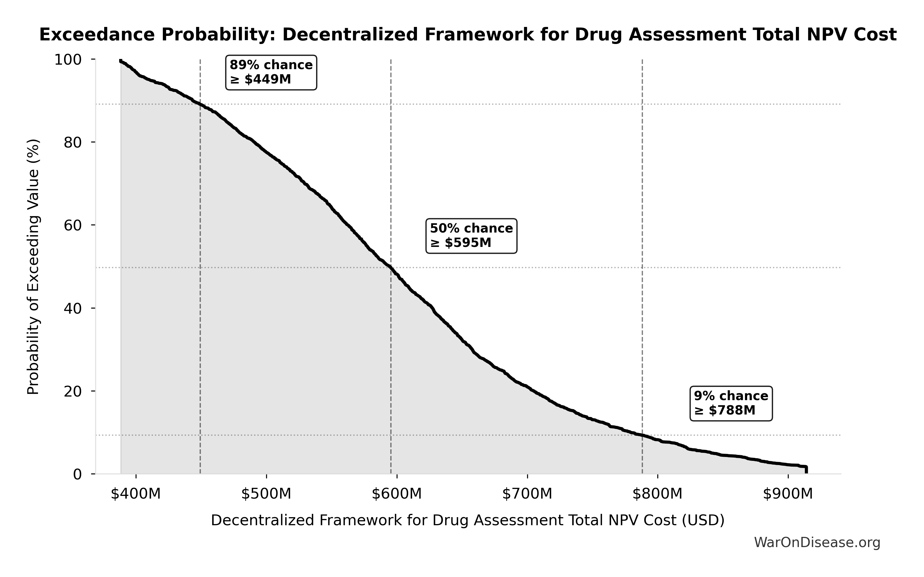
Exceedance Probability
This exceedance probability chart shows the likelihood that Decentralized Framework for Drug Assessment Total NPV Cost will exceed any given threshold. Higher curves indicate more favorable outcomes with greater certainty.
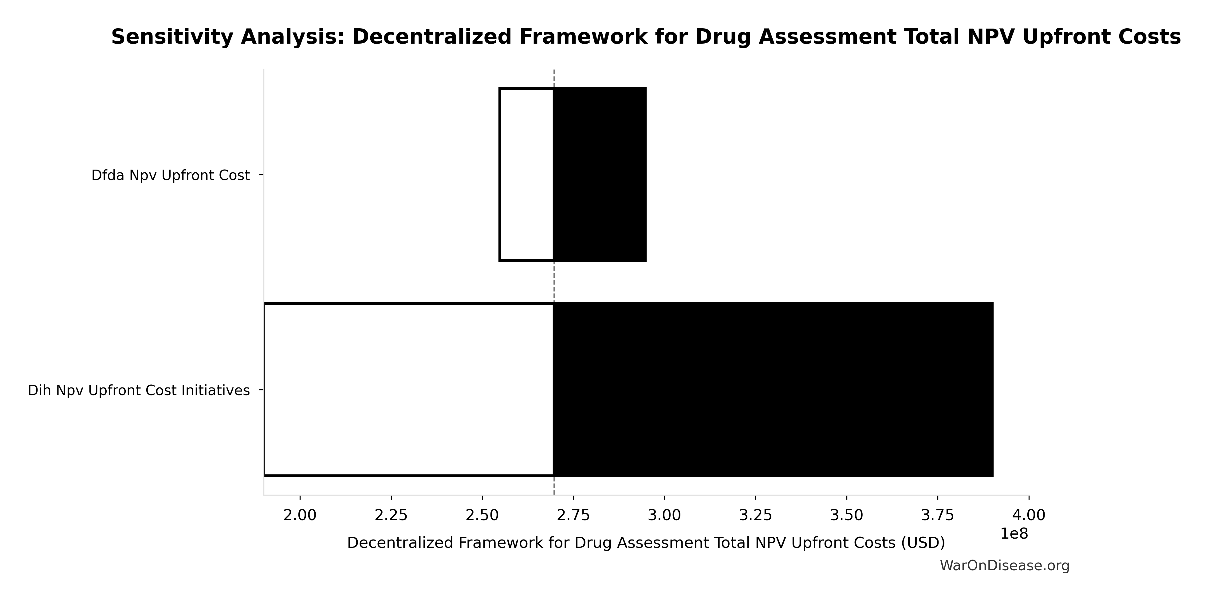
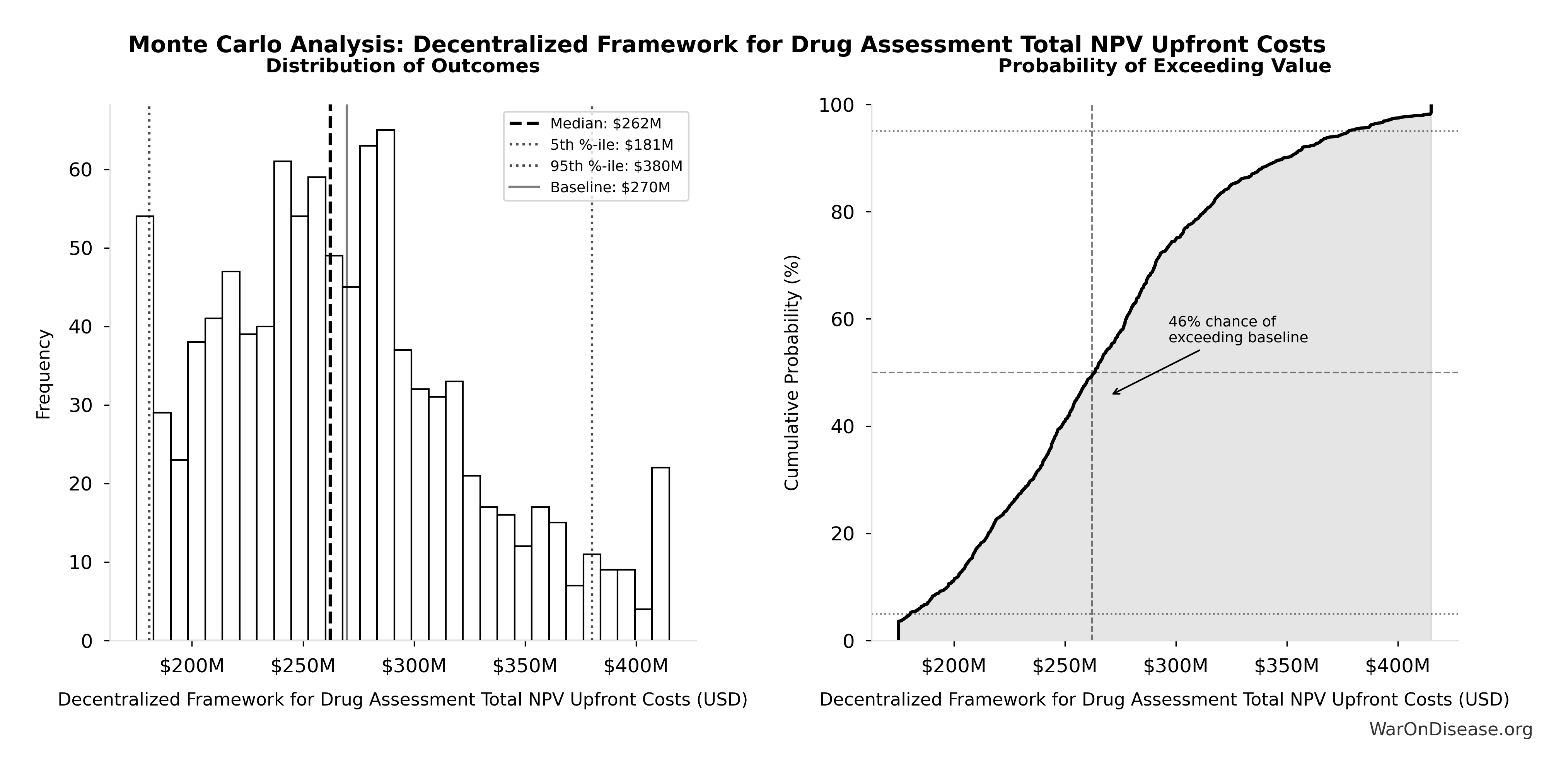
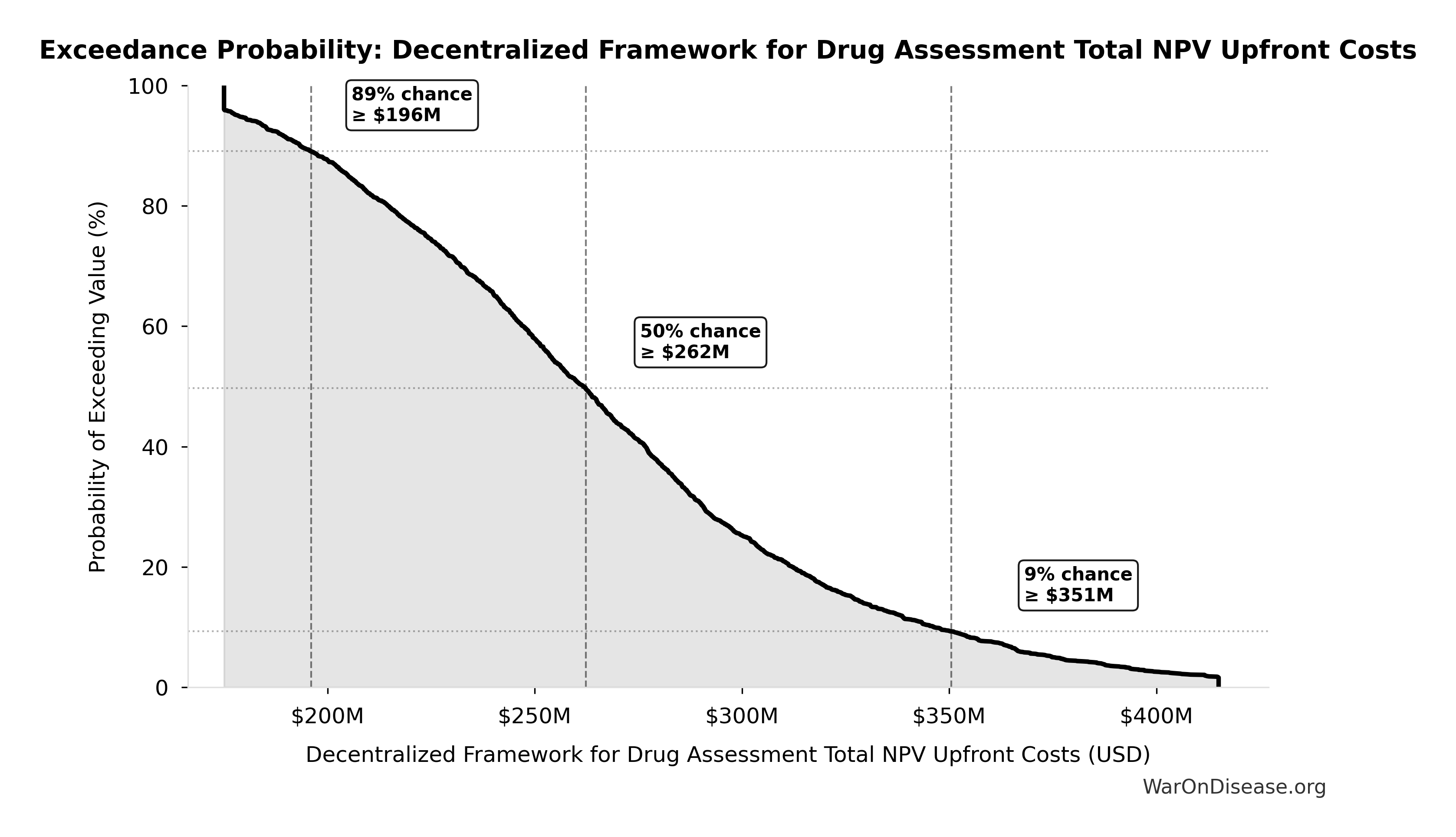
Decentralized Framework for Drug Assessment Total NPV Upfront Costs: $270M
Note📊 Details
Total NPV upfront costs (Decentralized Framework for Drug Assessment core + DIH initiatives)
Inputs:
- Decentralized Framework for Drug Assessment Core framework Build Cost: $40M (95% CI: $25M - $65M)
- DIH Broader Initiatives Upfront Cost: $230M (95% CI: $150M - $350M)
\[ \begin{gathered} Cost_{upfront,total} \\ = Cost_{upfront} + Cost_{DIH,init} \\ = \$40M + \$230M \\ = \$270M \end{gathered} \]
✓ High confidence
Sensitivity Analysis
Sensitivity Indices for Decentralized Framework for Drug Assessment Total NPV Upfront Costs
Regression-based sensitivity showing which inputs explain the most variance in the output.
| Input Parameter | Sensitivity Coefficient | Interpretation |
|---|---|---|
| DIH Broader Initiatives Upfront Cost (USD) | 0.8338 | Strong driver |
| Decentralized Framework for Drug Assessment Core framework Build Cost (USD) | 0.1662 | Weak driver |
Interpretation: Standardized coefficients show the change in output (in SD units) per 1 SD change in input. Values near ±1 indicate strong influence; values exceeding ±1 may occur with correlated inputs.
Monte Carlo Distribution
Simulation Results Summary: Decentralized Framework for Drug Assessment Total NPV Upfront Costs
| Statistic | Value |
|---|---|
| Baseline (deterministic) | $270M |
| Mean (expected value) | $269M |
| Median (50th percentile) | $262M |
| Standard Deviation | $58.1M |
| 90% Range (5th-95th percentile) | [$181M, $380M] |
The histogram shows the distribution of Decentralized Framework for Drug Assessment Total NPV Upfront Costs across 10,000 Monte Carlo simulations. The CDF (right) shows the probability of the outcome exceeding any given value, which is useful for risk assessment.
Exceedance Probability
This exceedance probability chart shows the likelihood that Decentralized Framework for Drug Assessment Total NPV Upfront Costs will exceed any given threshold. Higher curves indicate more favorable outcomes with greater certainty.
Decentralized Framework for Drug Assessment Overhead Percentage of Treaty Funding: 0.147%
Note📊 Details
Percentage of treaty funding allocated to Decentralized Framework for Drug Assessment framework overhead
Inputs:
- Total Annual Decentralized Framework for Drug Assessment Operational Costs 🔢: $40M
- Annual Funding from 1% of Global Military Spending Redirected to DIH 🔢: $27.2B
\[ \begin{gathered} OPEX_{pct} \\ = \frac{OPEX_{dFDA}}{Funding_{treaty}} \\ = \frac{\$40M}{\$27.2B} \\ = 0.147\% \end{gathered} \] where: \[ \begin{gathered} OPEX_{dFDA} \\ = Cost_{platform} + Cost_{staff} + Cost_{infra} \\ + Cost_{regulatory} + Cost_{community} \\ = \$15M + \$10M + \$8M + \$5M + \$2M \\ = \$40M \end{gathered} \] where: \[ \begin{gathered} Funding_{treaty} \\ = Spending_{mil} \times Reduce_{treaty} \\ = \$2.72T \times 1\% \\ = \$27.2B \end{gathered} \] ✓ High confidence
Sensitivity Analysis
Sensitivity Indices for Decentralized Framework for Drug Assessment Overhead Percentage of Treaty Funding
Regression-based sensitivity showing which inputs explain the most variance in the output.
| Input Parameter | Sensitivity Coefficient | Interpretation |
|---|---|---|
| Total Annual Decentralized Framework for Drug Assessment Operational Costs (USD/year) | 1.0000 | Strong driver |
Interpretation: Standardized coefficients show the change in output (in SD units) per 1 SD change in input. Values near ±1 indicate strong influence; values exceeding ±1 may occur with correlated inputs.
Monte Carlo Distribution
Simulation Results Summary: Decentralized Framework for Drug Assessment Overhead Percentage of Treaty Funding
| Statistic | Value |
|---|---|
| Baseline (deterministic) | 0.147% |
| Mean (expected value) | 0.147% |
| Median (50th percentile) | 0.143% |
| Standard Deviation | 0.0302% |
| 90% Range (5th-95th percentile) | [0.1%, 0.204%] |
The histogram shows the distribution of Decentralized Framework for Drug Assessment Overhead Percentage of Treaty Funding across 10,000 Monte Carlo simulations. The CDF (right) shows the probability of the outcome exceeding any given value, which is useful for risk assessment.
Exceedance Probability
This exceedance probability chart shows the likelihood that Decentralized Framework for Drug Assessment Overhead Percentage of Treaty Funding will exceed any given threshold. Higher curves indicate more favorable outcomes with greater certainty.
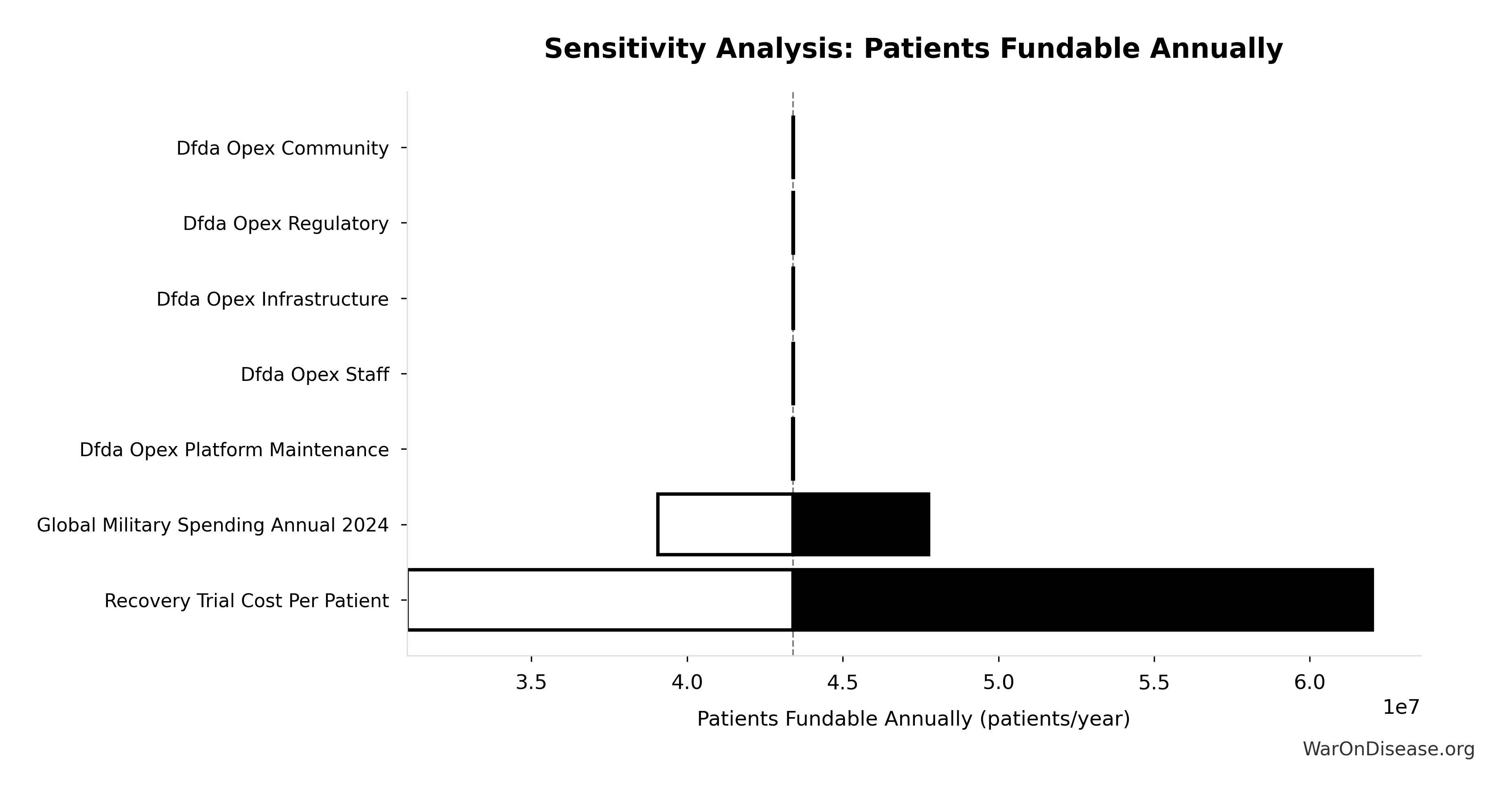
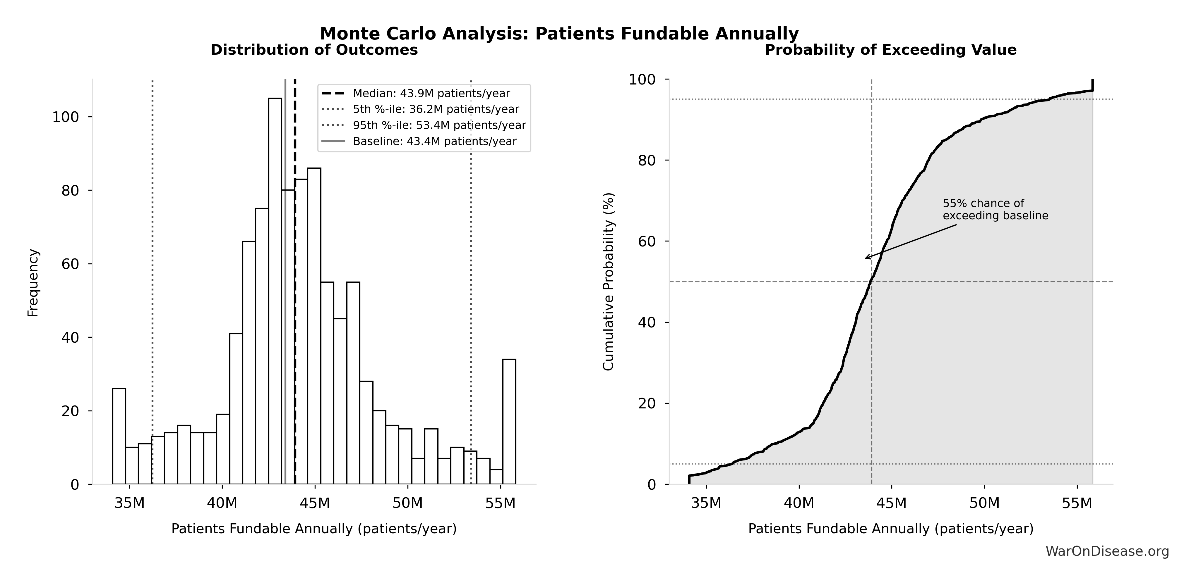
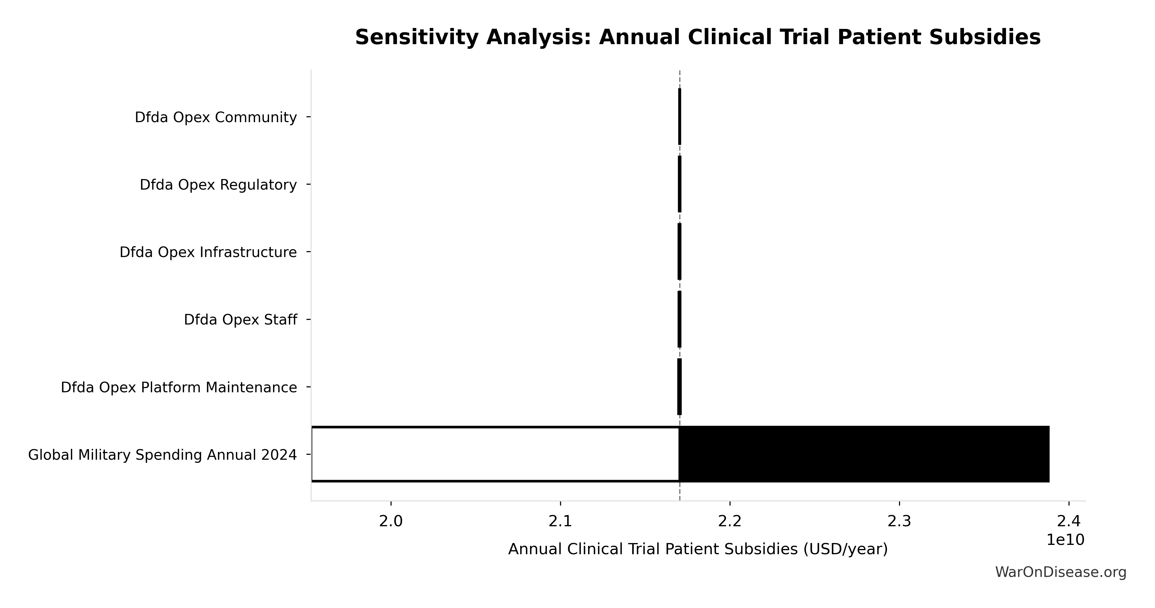
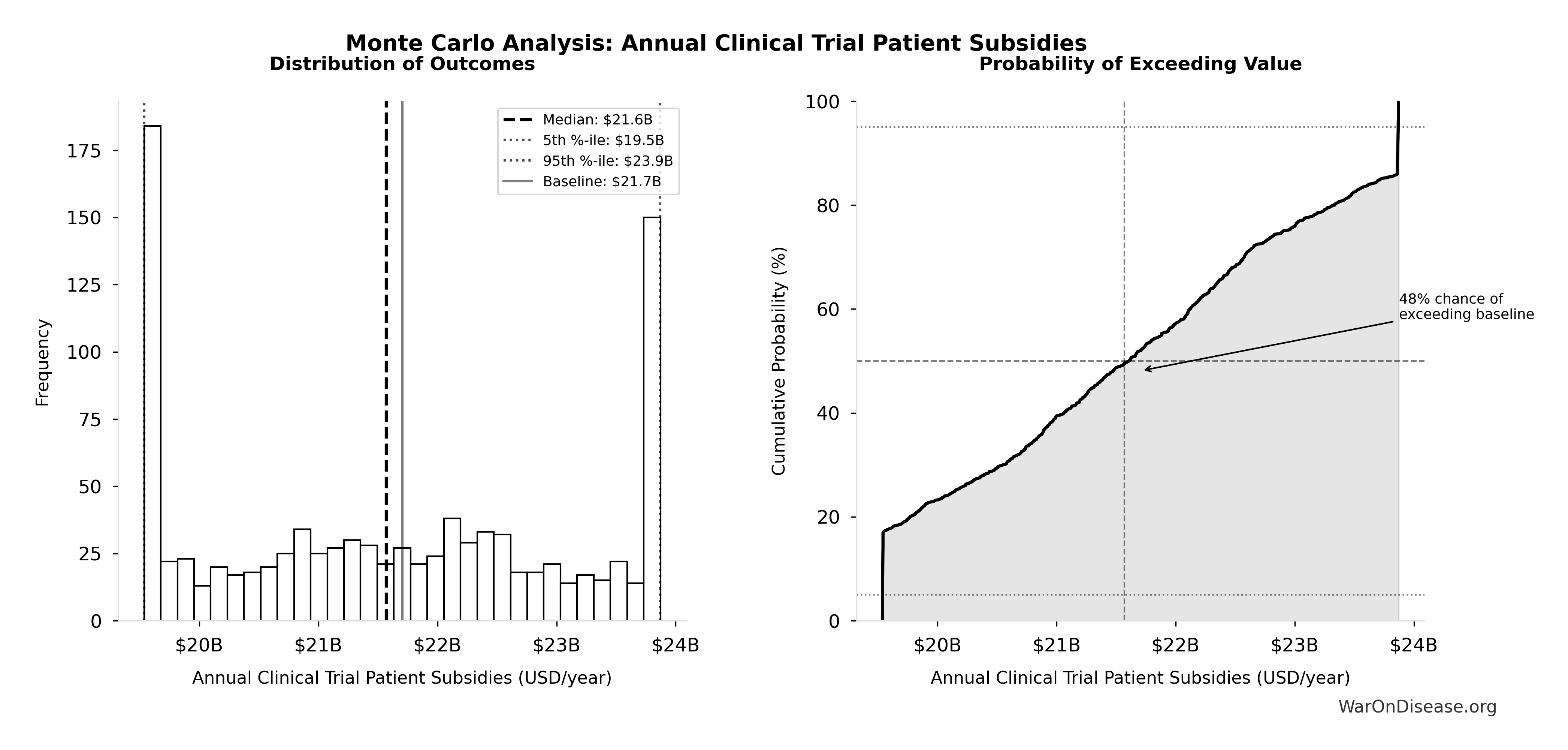
dFDA Patients Fundable Annually: 23.4 million patients/year
Note📊 Details
Number of patients fundable annually from dFDA funding at pragmatic trial cost. Source-agnostic counterpart of DIH_PATIENTS_FUNDABLE_ANNUALLY.
Inputs:
- dFDA Annual Trial Subsidies 🔢: $21.8B
- dFDA Pragmatic Trial Cost per Patient 📊: $929 (95% CI: $97 - $3K)
\[ \begin{gathered} N_{fundable,dFDA} \\ = \frac{Subsidies_{dFDA,ann}}{Cost_{pragmatic,pt}} \\ = \frac{\$21.8B}{\$929} \\ = 23.4M \end{gathered} \] where: \[ \begin{gathered} Subsidies_{dFDA,ann} \\ = Funding_{dFDA,ann} - OPEX_{dFDA} \\ = \$21.8B - \$40M \\ = \$21.8B \end{gathered} \] where: \[ \begin{gathered} OPEX_{dFDA} \\ = Cost_{platform} + Cost_{staff} + Cost_{infra} \\ + Cost_{regulatory} + Cost_{community} \\ = \$15M + \$10M + \$8M + \$5M + \$2M \\ = \$40M \end{gathered} \] ✓ High confidence
Sensitivity Analysis
Sensitivity Indices for dFDA Patients Fundable Annually
Regression-based sensitivity showing which inputs explain the most variance in the output.
| Input Parameter | Sensitivity Coefficient | Interpretation |
|---|---|---|
| dFDA Annual Trial Subsidies (USD/year) | 2.3351 | Strong driver |
| dFDA Pragmatic Trial Cost per Patient (USD/patient) | 1.5755 | Strong driver |
Interpretation: Standardized coefficients show the change in output (in SD units) per 1 SD change in input. Values near ±1 indicate strong influence; values exceeding ±1 may occur with correlated inputs.
Monte Carlo Distribution
Simulation Results Summary: dFDA Patients Fundable Annually
| Statistic | Value |
|---|---|
| Baseline (deterministic) | 23.4 million |
| Mean (expected value) | 38.6 million |
| Median (50th percentile) | 30.2 million |
| Standard Deviation | 30.2 million |
| 90% Range (5th-95th percentile) | [9.46 million, 97 million] |
The histogram shows the distribution of dFDA Patients Fundable Annually across 10,000 Monte Carlo simulations. The CDF (right) shows the probability of the outcome exceeding any given value, which is useful for risk assessment.
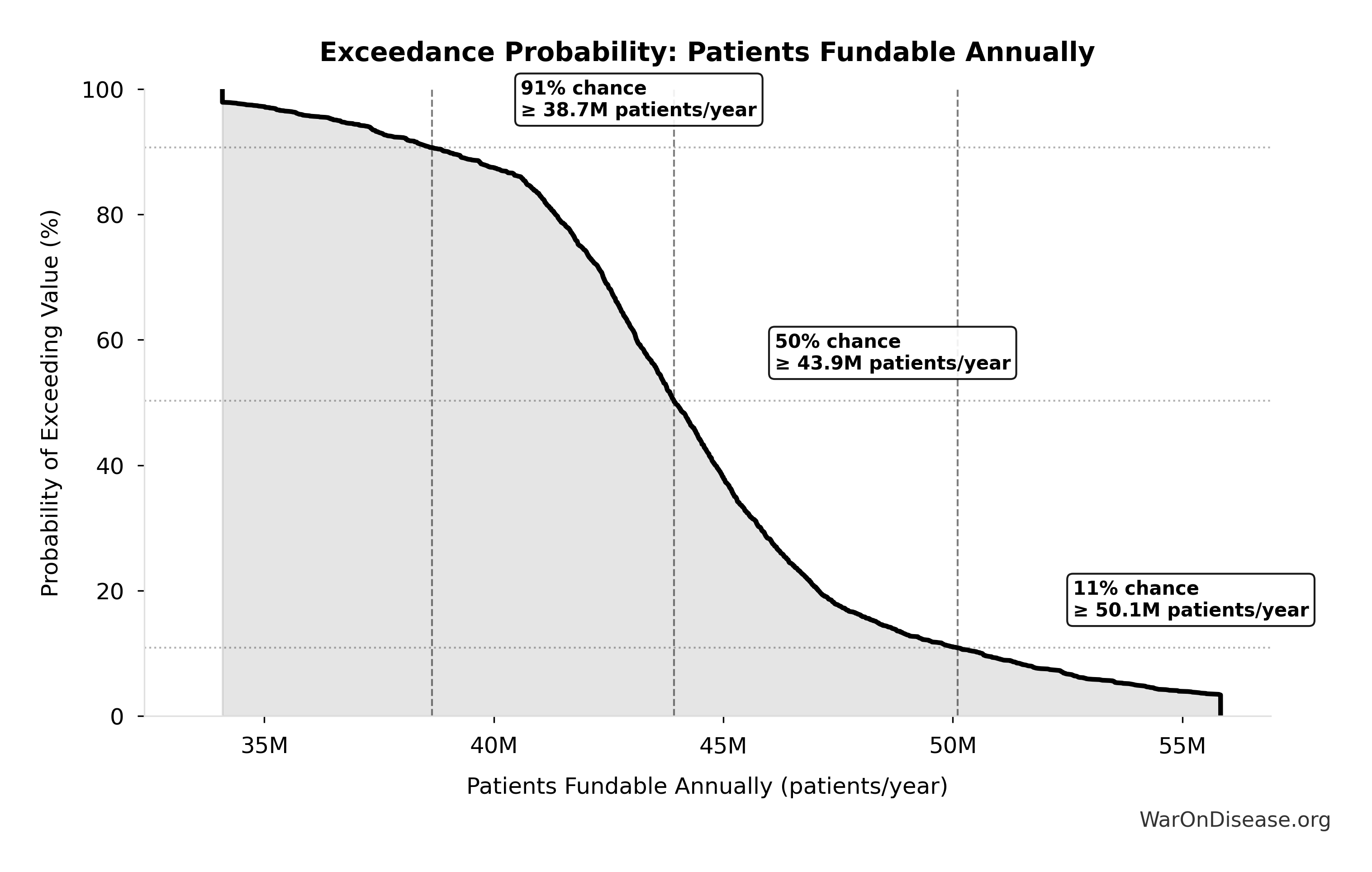
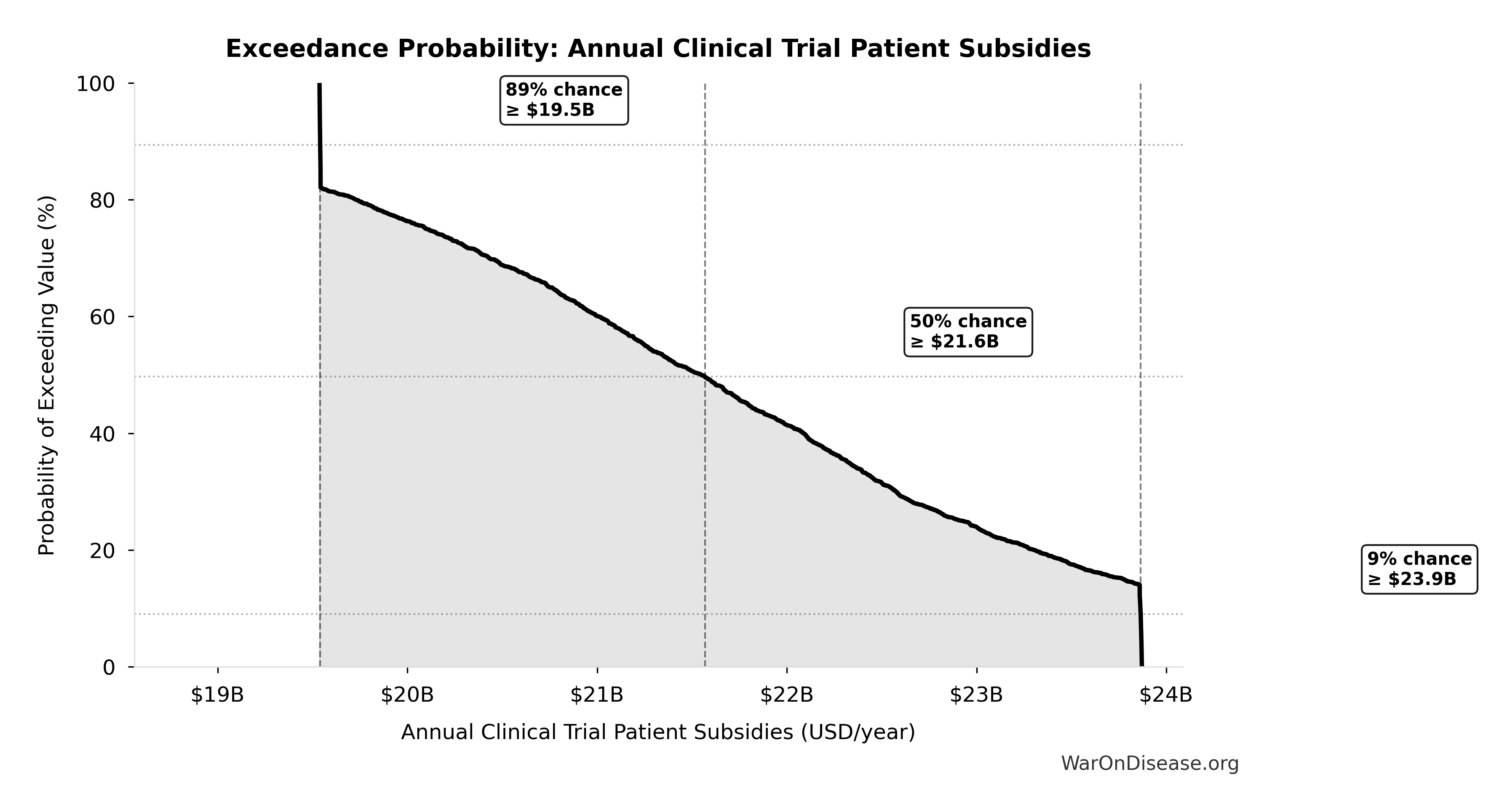
Exceedance Probability
This exceedance probability chart shows the likelihood that dFDA Patients Fundable Annually will exceed any given threshold. Higher curves indicate more favorable outcomes with greater certainty.
dFDA Therapeutic Space Exploration Time: 36 years
Note📊 Details
Years to explore the entire therapeutic search space with dFDA implementation. At increased discovery rate, finding first treatments for all currently untreatable diseases takes ~36 years instead of ~443.
Inputs:
- Status Quo Therapeutic Space Exploration Time 🔢: 443 years
- Trial Capacity Multiplier 🔢: 12.3x
\[ \begin{gathered} T_{queue,dFDA} \\ = \frac{T_{queue,SQ}}{k_{capacity}} \\ = \frac{443}{12.3} \\ = 36 \end{gathered} \] where: \[ \begin{gathered} T_{queue,SQ} \\ = \frac{N_{untreated}}{Treatments_{new,ann}} \\ = \frac{6{,}650}{15} \\ = 443 \end{gathered} \] where: \[ \begin{gathered} N_{untreated} \\ = N_{rare} \times 0.95 \\ = 7{,}000 \times 0.95 \\ = 6{,}650 \end{gathered} \] where: \[ \begin{gathered} k_{capacity} \\ = \frac{N_{fundable,dFDA}}{Slots_{curr}} \\ = \frac{23.4M}{1.9M} \\ = 12.3 \end{gathered} \] where: \[ \begin{gathered} N_{fundable,dFDA} \\ = \frac{Subsidies_{dFDA,ann}}{Cost_{pragmatic,pt}} \\ = \frac{\$21.8B}{\$929} \\ = 23.4M \end{gathered} \] where: \[ \begin{gathered} Subsidies_{dFDA,ann} \\ = Funding_{dFDA,ann} - OPEX_{dFDA} \\ = \$21.8B - \$40M \\ = \$21.8B \end{gathered} \] where: \[ \begin{gathered} OPEX_{dFDA} \\ = Cost_{platform} + Cost_{staff} + Cost_{infra} \\ + Cost_{regulatory} + Cost_{community} \\ = \$15M + \$10M + \$8M + \$5M + \$2M \\ = \$40M \end{gathered} \] ? Low confidence
Sensitivity Analysis
Sensitivity Indices for dFDA Therapeutic Space Exploration Time
Regression-based sensitivity showing which inputs explain the most variance in the output.
| Input Parameter | Sensitivity Coefficient | Interpretation |
|---|---|---|
| Status Quo Therapeutic Space Exploration Time (years) | -1.3321 | Strong driver |
| Trial Capacity Multiplier (x) | 0.4867 | Moderate driver |
Interpretation: Standardized coefficients show the change in output (in SD units) per 1 SD change in input. Values near ±1 indicate strong influence; values exceeding ±1 may occur with correlated inputs.
Monte Carlo Distribution
Simulation Results Summary: dFDA Therapeutic Space Exploration Time
| Statistic | Value |
|---|---|
| Baseline (deterministic) | 36 |
| Mean (expected value) | 34.5 |
| Median (50th percentile) | 29.6 |
| Standard Deviation | 19.9 |
| 90% Range (5th-95th percentile) | [11.6, 77.1] |
The histogram shows the distribution of dFDA Therapeutic Space Exploration Time across 10,000 Monte Carlo simulations. The CDF (right) shows the probability of the outcome exceeding any given value, which is useful for risk assessment.
Exceedance Probability
This exceedance probability chart shows the likelihood that dFDA Therapeutic Space Exploration Time will exceed any given threshold. Higher curves indicate more favorable outcomes with greater certainty.
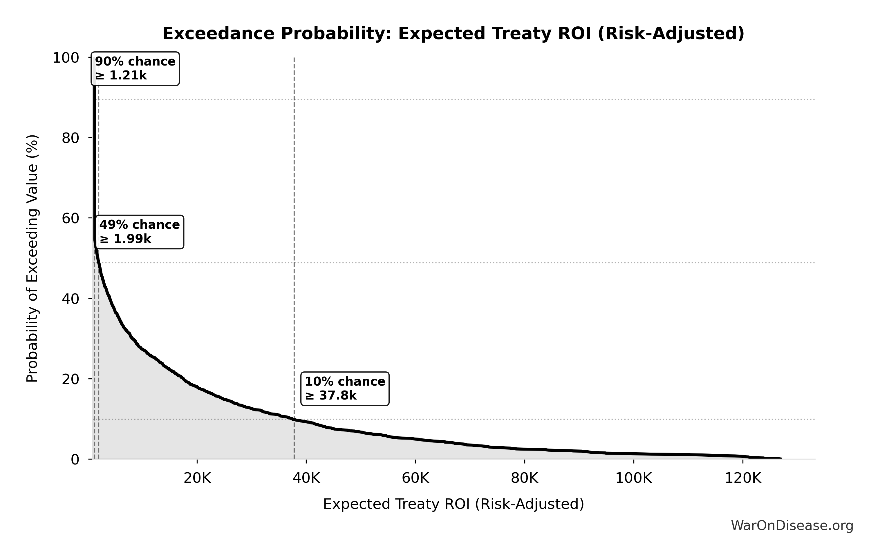
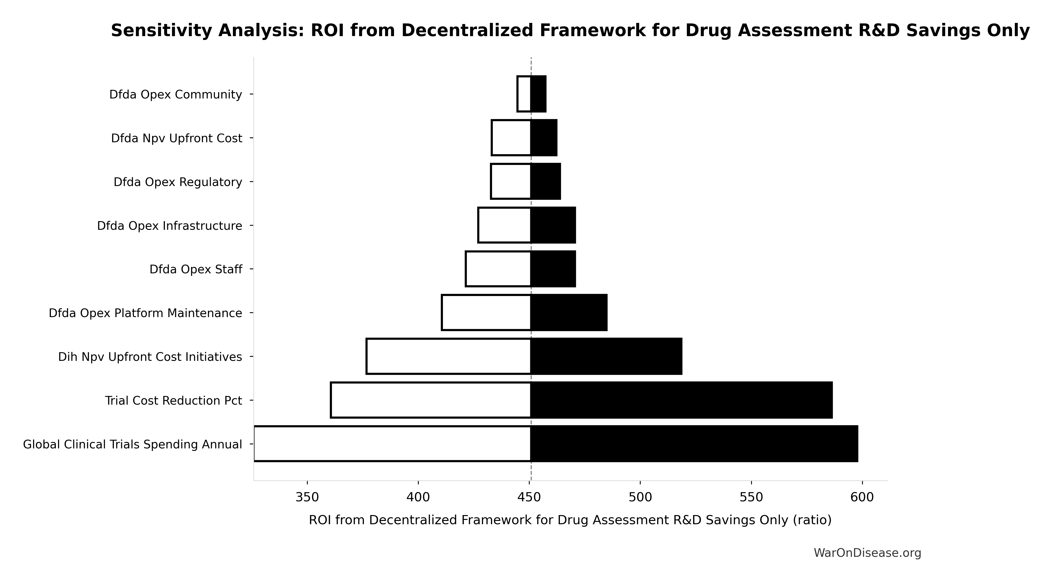
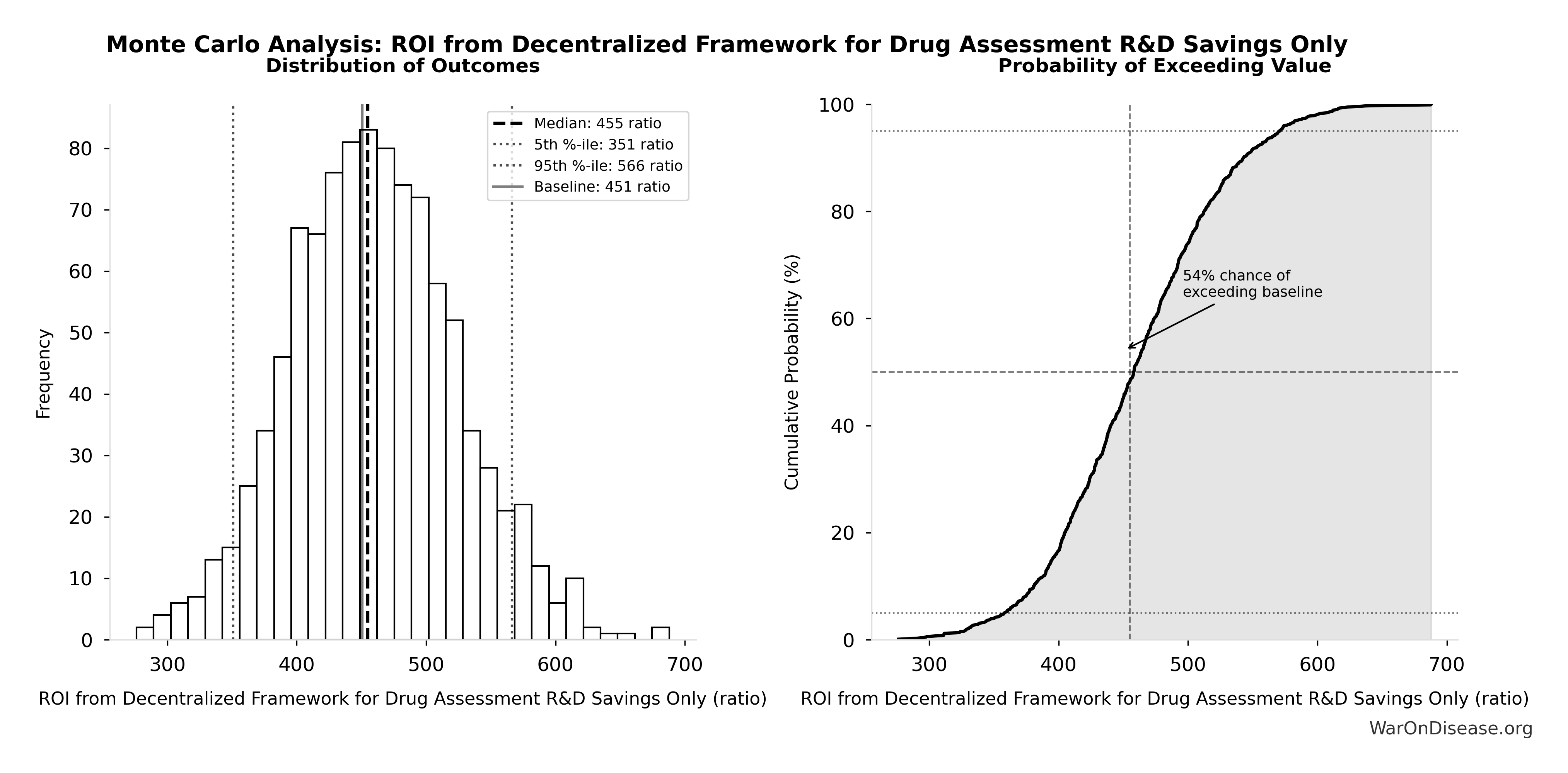
ROI from Decentralized Framework for Drug Assessment R&D Savings Only: 637:1
Note📊 Details
ROI from Decentralized Framework for Drug Assessment R&D savings only (10-year NPV, most conservative estimate)
Inputs:
- NPV of Decentralized Framework for Drug Assessment Benefits (R&D Only, 10-Year Discounted) 🔢: $389B
- Decentralized Framework for Drug Assessment Total NPV Cost 🔢: $611M
\[ \begin{gathered} ROI_{RD} \\ = \frac{NPV_{RD}}{Cost_{dFDA,total}} \\ = \frac{\$389B}{\$611M} \\ = 637 \end{gathered} \] where: \[ \begin{gathered} NPV_{RD} \\ = \sum_{t=1}^{10} \frac{Savings_{RD,ann} \times \frac{\min(t,5)}{5}}{(1+r)^t} \end{gathered} \] where: \[ \begin{gathered} Savings_{RD,ann} \\ = Benefit_{RD,ann} - OPEX_{dFDA} \\ = \$58.6B - \$40M \\ = \$58.6B \end{gathered} \] where: \[ \begin{gathered} Benefit_{RD,ann} \\ = Spending_{trials} \times Reduce_{pct} \\ = \$60B \times 97.7\% \\ = \$58.6B \end{gathered} \] where: \[ \begin{gathered} Reduce_{pct} \\ = 1 - \frac{Cost_{pragmatic,pt}}{Cost_{P3,pt}} \\ = 1 - \frac{\$929}{\$41K} \\ = 97.7\% \end{gathered} \] where: \[ \begin{gathered} OPEX_{dFDA} \\ = Cost_{platform} + Cost_{staff} + Cost_{infra} \\ + Cost_{regulatory} + Cost_{community} \\ = \$15M + \$10M + \$8M + \$5M + \$2M \\ = \$40M \end{gathered} \] where: \[ \begin{gathered} Cost_{dFDA,total} \\ = PV_{OPEX} + Cost_{upfront,total} \\ = \$342M + \$270M \\ = \$611M \end{gathered} \] where: \[ PV_{OPEX} = OPEX_{ann} \times \frac{1 - (1+r)^{-T}}{r} \] where: \[ \begin{gathered} OPEX_{total} \\ = OPEX_{ann} + OPEX_{DIH,ann} \\ = \$18.9M + \$21.1M \\ = \$40M \end{gathered} \] where: \[ \begin{gathered} Cost_{upfront,total} \\ = Cost_{upfront} + Cost_{DIH,init} \\ = \$40M + \$230M \\ = \$270M \end{gathered} \] ✓ High confidence
Sensitivity Analysis
Sensitivity Indices for ROI from Decentralized Framework for Drug Assessment R&D Savings Only
Regression-based sensitivity showing which inputs explain the most variance in the output.
| Input Parameter | Sensitivity Coefficient | Interpretation |
|---|---|---|
| Decentralized Framework for Drug Assessment Total NPV Cost (USD) | -2.6305 | Strong driver |
| NPV of Decentralized Framework for Drug Assessment Benefits (R&D Only, 10-Year Discounted) (USD) | 1.7615 | Strong driver |
Interpretation: Standardized coefficients show the change in output (in SD units) per 1 SD change in input. Values near ±1 indicate strong influence; values exceeding ±1 may occur with correlated inputs.
Monte Carlo Distribution
Simulation Results Summary: ROI from Decentralized Framework for Drug Assessment R&D Savings Only
| Statistic | Value |
|---|---|
| Baseline (deterministic) | 637:1 |
| Mean (expected value) | 653:1 |
| Median (50th percentile) | 645:1 |
| Standard Deviation | 58.4:1 |
| 90% Range (5th-95th percentile) | [569:1, 790:1] |
The histogram shows the distribution of ROI from Decentralized Framework for Drug Assessment R&D Savings Only across 10,000 Monte Carlo simulations. The CDF (right) shows the probability of the outcome exceeding any given value, which is useful for risk assessment.
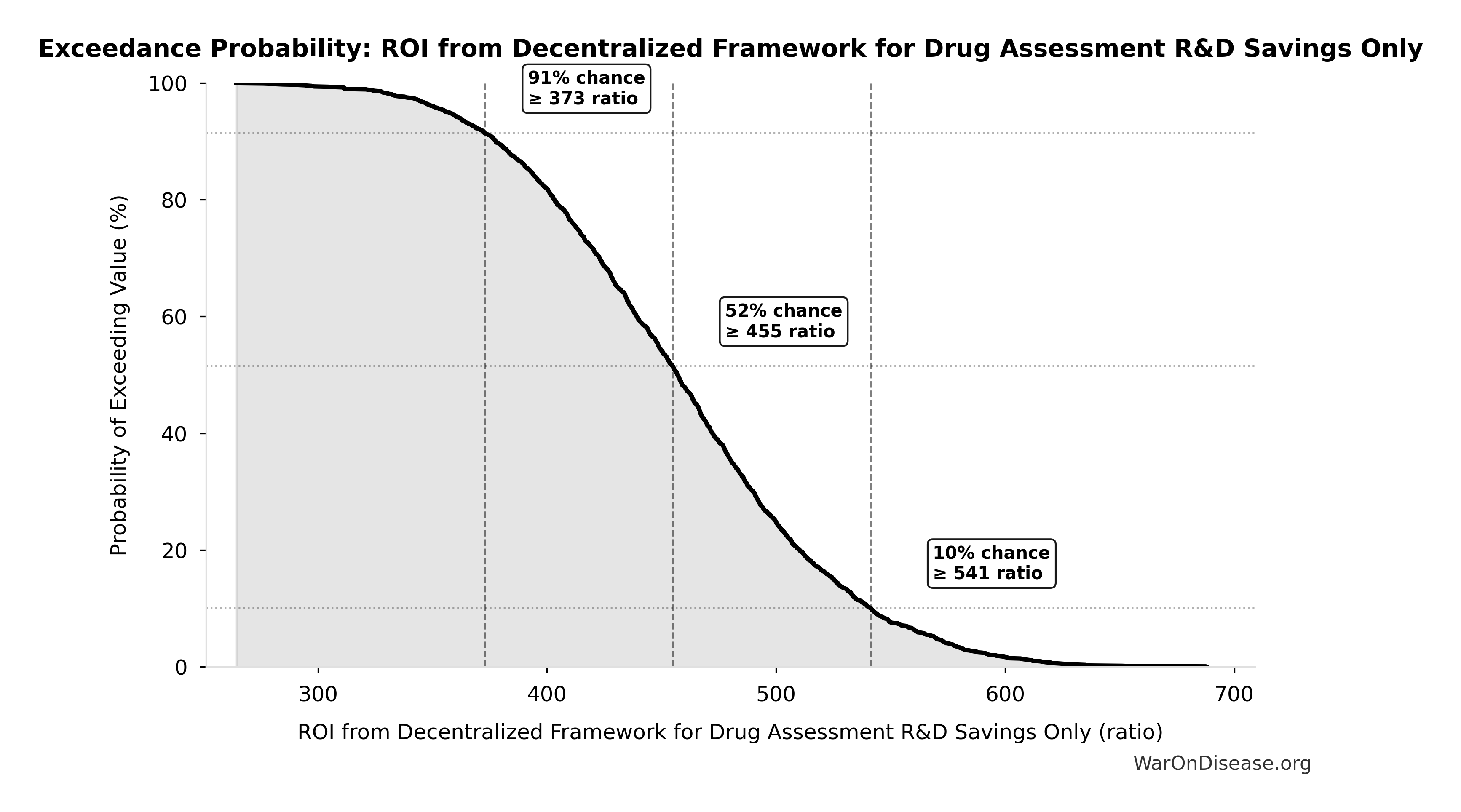
Exceedance Probability
This exceedance probability chart shows the likelihood that ROI from Decentralized Framework for Drug Assessment R&D Savings Only will exceed any given threshold. Higher curves indicate more favorable outcomes with greater certainty.
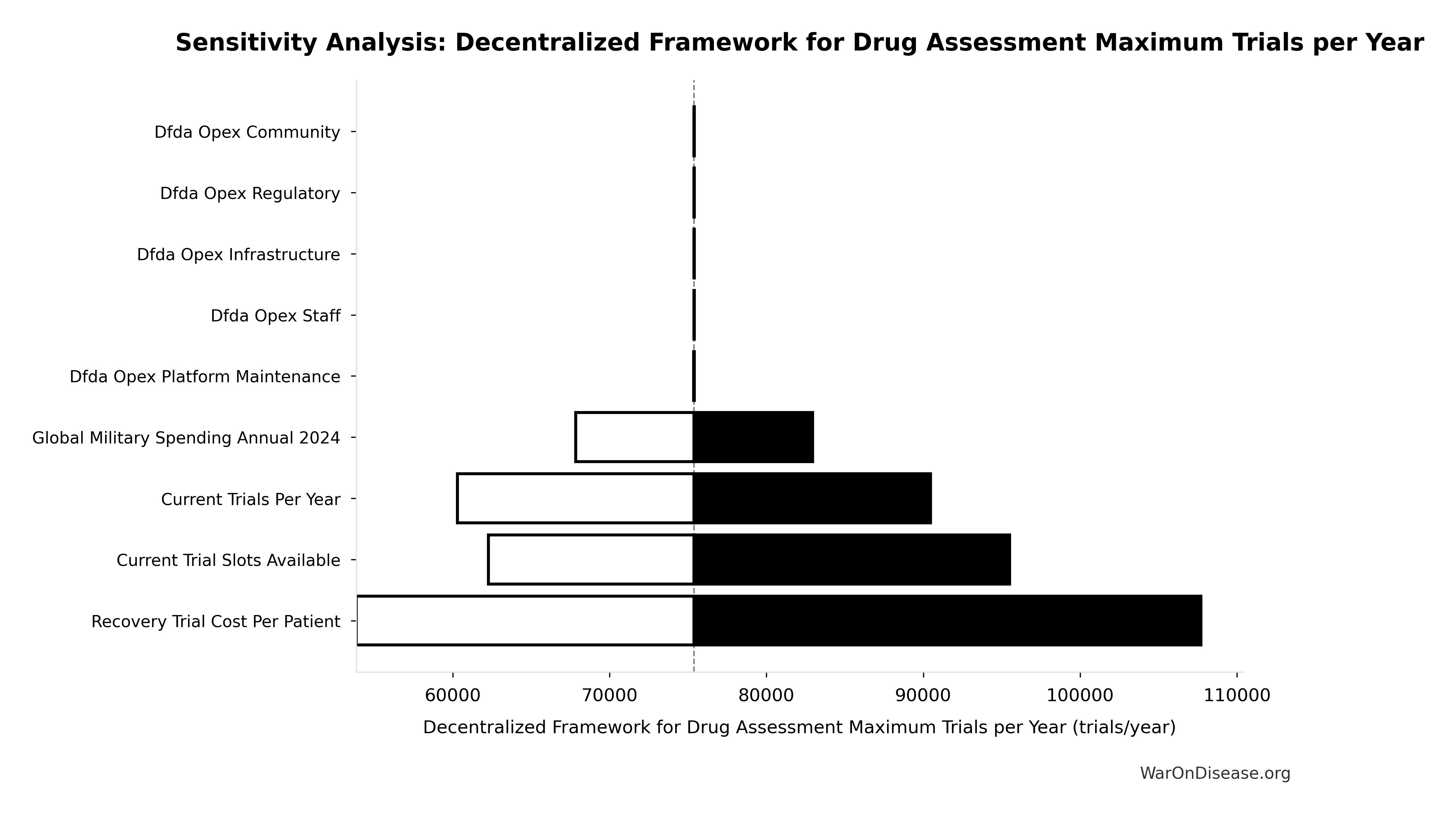
Decentralized Framework for Drug Assessment Maximum Trials per Year: 40.7 thousand trials/year
Note📊 Details
Maximum trials per year possible with trial capacity multiplier
Inputs:
- Current Global Clinical Trials per Year 📊: 3.3 thousand trials/year (95% CI: 2.64 thousand trials/year - 3.96 thousand trials/year)
- Trial Capacity Multiplier 🔢: 12.3x
\[ \begin{gathered} Capacity_{trials} \\ = Trials_{ann,curr} \times k_{capacity} \\ = 3{,}300 \times 12.3 \\ = 40{,}700 \end{gathered} \] where: \[ \begin{gathered} k_{capacity} \\ = \frac{N_{fundable,dFDA}}{Slots_{curr}} \\ = \frac{23.4M}{1.9M} \\ = 12.3 \end{gathered} \] where: \[ \begin{gathered} N_{fundable,dFDA} \\ = \frac{Subsidies_{dFDA,ann}}{Cost_{pragmatic,pt}} \\ = \frac{\$21.8B}{\$929} \\ = 23.4M \end{gathered} \] where: \[ \begin{gathered} Subsidies_{dFDA,ann} \\ = Funding_{dFDA,ann} - OPEX_{dFDA} \\ = \$21.8B - \$40M \\ = \$21.8B \end{gathered} \] where: \[ \begin{gathered} OPEX_{dFDA} \\ = Cost_{platform} + Cost_{staff} + Cost_{infra} \\ + Cost_{regulatory} + Cost_{community} \\ = \$15M + \$10M + \$8M + \$5M + \$2M \\ = \$40M \end{gathered} \] ✓ High confidence
Sensitivity Analysis
Sensitivity Indices for Decentralized Framework for Drug Assessment Maximum Trials per Year
Regression-based sensitivity showing which inputs explain the most variance in the output.
| Input Parameter | Sensitivity Coefficient | Interpretation |
|---|---|---|
| Trial Capacity Multiplier (x) | 0.9321 | Strong driver |
| Current Global Clinical Trials per Year (trials/year) | -0.0802 | Minimal effect |
Interpretation: Standardized coefficients show the change in output (in SD units) per 1 SD change in input. Values near ±1 indicate strong influence; values exceeding ±1 may occur with correlated inputs.
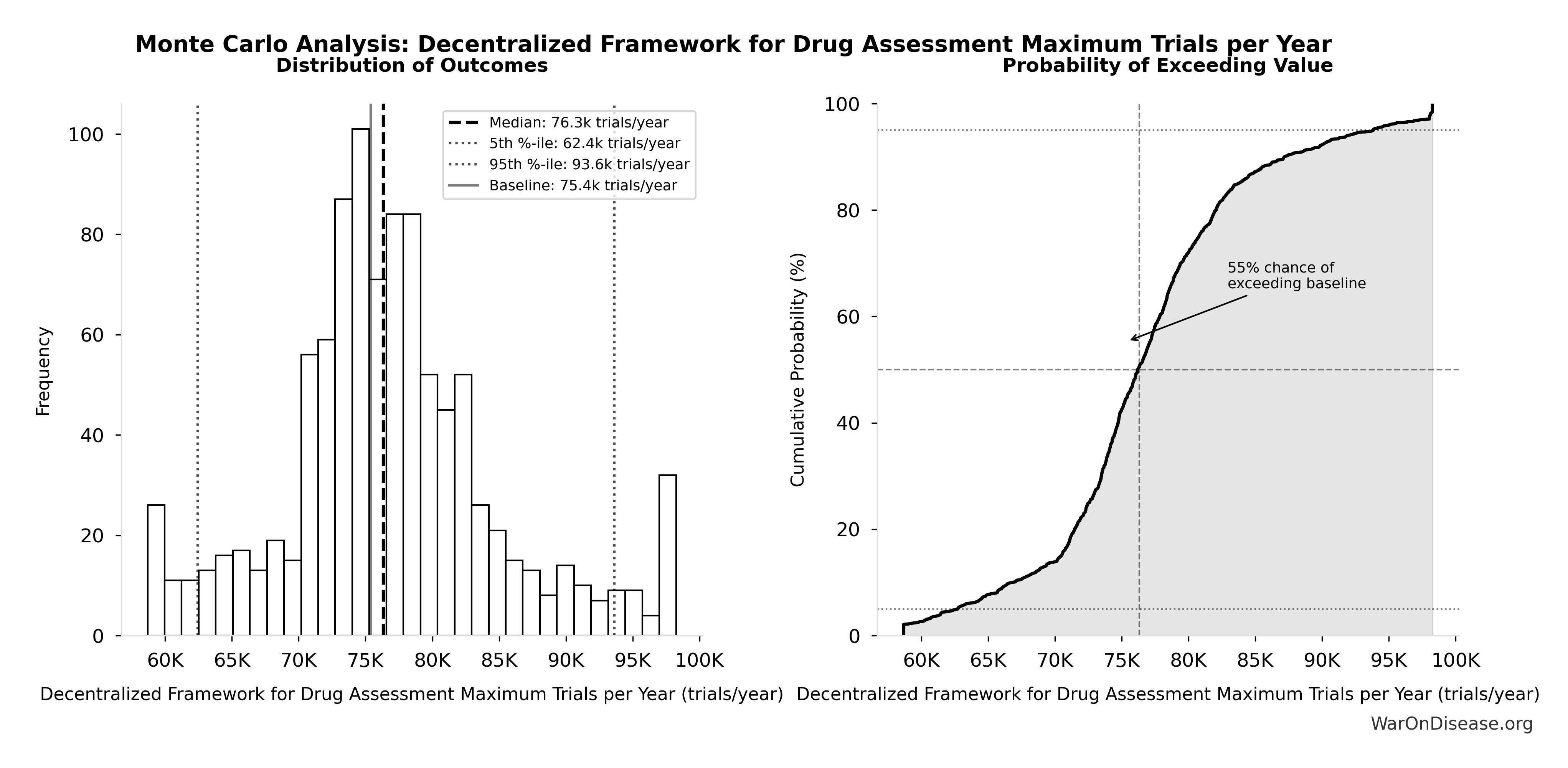
Monte Carlo Distribution
Simulation Results Summary: Decentralized Framework for Drug Assessment Maximum Trials per Year
| Statistic | Value |
|---|---|
| Baseline (deterministic) | 40.7 thousand |
| Mean (expected value) | 67.4 thousand |
| Median (50th percentile) | 52.5 thousand |
| Standard Deviation | 53.2 thousand |
| 90% Range (5th-95th percentile) | [16.3 thousand, 170 thousand] |
The histogram shows the distribution of Decentralized Framework for Drug Assessment Maximum Trials per Year across 10,000 Monte Carlo simulations. The CDF (right) shows the probability of the outcome exceeding any given value, which is useful for risk assessment.
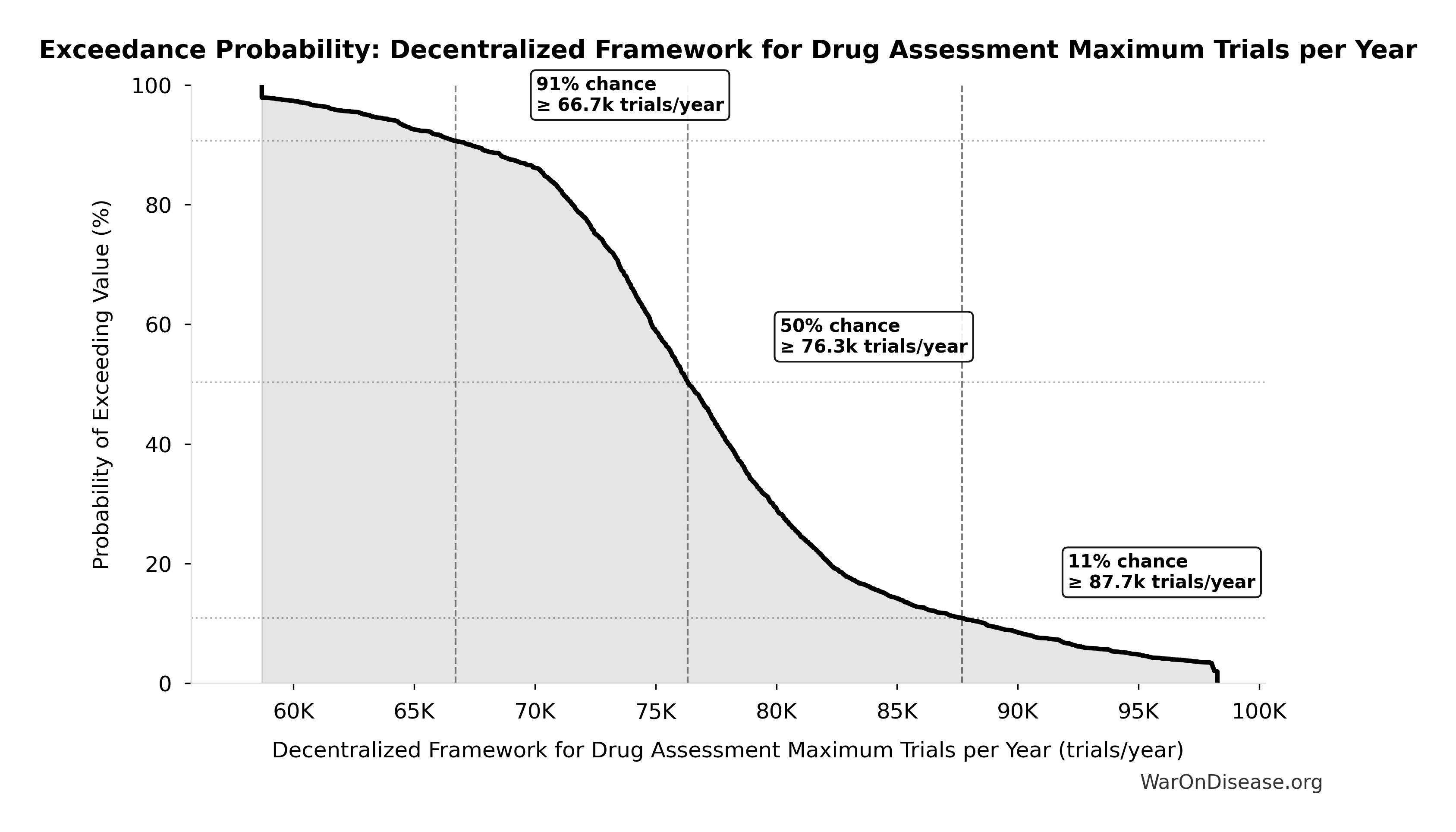
Exceedance Probability
This exceedance probability chart shows the likelihood that Decentralized Framework for Drug Assessment Maximum Trials per Year will exceed any given threshold. Higher curves indicate more favorable outcomes with greater certainty.
Trial Capacity Multiplier: 12.3x
Note📊 Details
Trial capacity multiplier from dFDA funding capacity vs. current global trial participation
Inputs:
- Annual Global Clinical Trial Participants 📊: 1.9 million patients/year (95% CI: 1.5 million patients/year - 2.3 million patients/year)
- dFDA Patients Fundable Annually 🔢: 23.4 million patients/year
\[ \begin{gathered} k_{capacity} \\ = \frac{N_{fundable,dFDA}}{Slots_{curr}} \\ = \frac{23.4M}{1.9M} \\ = 12.3 \end{gathered} \] where: \[ \begin{gathered} N_{fundable,dFDA} \\ = \frac{Subsidies_{dFDA,ann}}{Cost_{pragmatic,pt}} \\ = \frac{\$21.8B}{\$929} \\ = 23.4M \end{gathered} \] where: \[ \begin{gathered} Subsidies_{dFDA,ann} \\ = Funding_{dFDA,ann} - OPEX_{dFDA} \\ = \$21.8B - \$40M \\ = \$21.8B \end{gathered} \] where: \[ \begin{gathered} OPEX_{dFDA} \\ = Cost_{platform} + Cost_{staff} + Cost_{infra} \\ + Cost_{regulatory} + Cost_{community} \\ = \$15M + \$10M + \$8M + \$5M + \$2M \\ = \$40M \end{gathered} \] ✓ High confidence
Sensitivity Analysis
Sensitivity Indices for Trial Capacity Multiplier
Regression-based sensitivity showing which inputs explain the most variance in the output.
| Input Parameter | Sensitivity Coefficient | Interpretation |
|---|---|---|
| dFDA Patients Fundable Annually (patients/year) | 1.0768 | Strong driver |
| Annual Global Clinical Trial Participants (patients/year) | 0.0910 | Minimal effect |
Interpretation: Standardized coefficients show the change in output (in SD units) per 1 SD change in input. Values near ±1 indicate strong influence; values exceeding ±1 may occur with correlated inputs.
Monte Carlo Distribution
Simulation Results Summary: Trial Capacity Multiplier
| Statistic | Value |
|---|---|
| Baseline (deterministic) | 12.3x |
| Mean (expected value) | 22.1x |
| Median (50th percentile) | 16x |
| Standard Deviation | 20.2x |
| 90% Range (5th-95th percentile) | [4.2x, 61.4x] |
The histogram shows the distribution of Trial Capacity Multiplier across 10,000 Monte Carlo simulations. The CDF (right) shows the probability of the outcome exceeding any given value, which is useful for risk assessment.
Exceedance Probability
This exceedance probability chart shows the likelihood that Trial Capacity Multiplier will exceed any given threshold. Higher curves indicate more favorable outcomes with greater certainty.
Total DALYs from Elimination of Efficacy Lag Plus Earlier Treatment Discovery from Higher Trial Throughput: 565 billion DALYs
Note📊 Details
Total DALYs averted from the combined dFDA timeline shift. Calculated as annual global DALY burden × eventually avoidable percentage × timeline shift years. Includes both fatal and non-fatal diseases (WHO GBD methodology).
Inputs:
- Global Annual DALY Burden 📊: 2.88 billion DALYs/year (SE: ±150 million DALYs/year)
- Eventually Avoidable DALY Percentage: 92.6% (95% CI: 50% - 98%)
- dFDA Average Total Timeline Shift 🔢: 212 years
\[ \begin{gathered} DALYs_{max} \\ = DALYs_{global,ann} \times Pct_{avoid,DALY} \times T_{accel,max} \\ = 2.88B \times 92.6\% \times 212 \\ = 565B \end{gathered} \] where: \[ T_{accel,max} = T_{accel} + T_{lag} = 204 + 8.2 = 212 \] where: \[ \begin{gathered} T_{accel} \\ = T_{first,SQ} \times \left(1 - \frac{1}{k_{capacity}}\right) \\ = 222 \times \left(1 - \frac{1}{12.3}\right) \\ = 204 \end{gathered} \] where: \[ \begin{gathered} T_{first,SQ} \\ = T_{queue,SQ} \times 0.5 \\ = 443 \times 0.5 \\ = 222 \end{gathered} \] where: \[ \begin{gathered} T_{queue,SQ} \\ = \frac{N_{untreated}}{Treatments_{new,ann}} \\ = \frac{6{,}650}{15} \\ = 443 \end{gathered} \] where: \[ \begin{gathered} N_{untreated} \\ = N_{rare} \times 0.95 \\ = 7{,}000 \times 0.95 \\ = 6{,}650 \end{gathered} \] where: \[ \begin{gathered} k_{capacity} \\ = \frac{N_{fundable,dFDA}}{Slots_{curr}} \\ = \frac{23.4M}{1.9M} \\ = 12.3 \end{gathered} \] where: \[ \begin{gathered} N_{fundable,dFDA} \\ = \frac{Subsidies_{dFDA,ann}}{Cost_{pragmatic,pt}} \\ = \frac{\$21.8B}{\$929} \\ = 23.4M \end{gathered} \] where: \[ \begin{gathered} Subsidies_{dFDA,ann} \\ = Funding_{dFDA,ann} - OPEX_{dFDA} \\ = \$21.8B - \$40M \\ = \$21.8B \end{gathered} \] where: \[ \begin{gathered} OPEX_{dFDA} \\ = Cost_{platform} + Cost_{staff} + Cost_{infra} \\ + Cost_{regulatory} + Cost_{community} \\ = \$15M + \$10M + \$8M + \$5M + \$2M \\ = \$40M \end{gathered} \] ? Low confidence
Sensitivity Analysis
Sensitivity Indices for Total DALYs from Elimination of Efficacy Lag Plus Earlier Treatment Discovery from Higher Trial Throughput
Regression-based sensitivity showing which inputs explain the most variance in the output.
| Input Parameter | Sensitivity Coefficient | Interpretation |
|---|---|---|
| dFDA Average Total Timeline Shift (years) | 0.8999 | Strong driver |
| Eventually Avoidable DALY Percentage (percentage) | 0.4866 | Moderate driver |
| Global Annual DALY Burden (DALYs/year) | 0.0432 | Minimal effect |
Interpretation: Standardized coefficients show the change in output (in SD units) per 1 SD change in input. Values near ±1 indicate strong influence; values exceeding ±1 may occur with correlated inputs.
Monte Carlo Distribution
Simulation Results Summary: Total DALYs from Elimination of Efficacy Lag Plus Earlier Treatment Discovery from Higher Trial Throughput
| Statistic | Value |
|---|---|
| Baseline (deterministic) | 565 billion |
| Mean (expected value) | 610 billion |
| Median (50th percentile) | 614 billion |
| Standard Deviation | 148 billion |
| 90% Range (5th-95th percentile) | [361 billion, 877 billion] |
The histogram shows the distribution of Total DALYs from Elimination of Efficacy Lag Plus Earlier Treatment Discovery from Higher Trial Throughput across 10,000 Monte Carlo simulations. The CDF (right) shows the probability of the outcome exceeding any given value, which is useful for risk assessment.
Exceedance Probability
This exceedance probability chart shows the likelihood that Total DALYs from Elimination of Efficacy Lag Plus Earlier Treatment Discovery from Higher Trial Throughput will exceed any given threshold. Higher curves indicate more favorable outcomes with greater certainty.
Total Economic Benefit from Elimination of Efficacy Lag Plus Earlier Treatment Discovery from Higher Trial Throughput: $84.8 quadrillion
Note📊 Details
Total economic value from the combined dFDA timeline shift. DALYs valued at standard economic rate.
Inputs:
- Total DALYs from Elimination of Efficacy Lag Plus Earlier Treatment Discovery from Higher Trial Throughput 🔢: 565 billion DALYs
- Standard Economic Value per QALY 📊: $150K (SE: ±$30K)
\[ \begin{gathered} Value_{max} \\ = DALYs_{max} \times Value_{QALY} \\ = 565B \times \$150K \\ = \$84800T \end{gathered} \] where: \[ \begin{gathered} DALYs_{max} \\ = DALYs_{global,ann} \times Pct_{avoid,DALY} \times T_{accel,max} \\ = 2.88B \times 92.6\% \times 212 \\ = 565B \end{gathered} \] where: \[ T_{accel,max} = T_{accel} + T_{lag} = 204 + 8.2 = 212 \] where: \[ \begin{gathered} T_{accel} \\ = T_{first,SQ} \times \left(1 - \frac{1}{k_{capacity}}\right) \\ = 222 \times \left(1 - \frac{1}{12.3}\right) \\ = 204 \end{gathered} \] where: \[ \begin{gathered} T_{first,SQ} \\ = T_{queue,SQ} \times 0.5 \\ = 443 \times 0.5 \\ = 222 \end{gathered} \] where: \[ \begin{gathered} T_{queue,SQ} \\ = \frac{N_{untreated}}{Treatments_{new,ann}} \\ = \frac{6{,}650}{15} \\ = 443 \end{gathered} \] where: \[ \begin{gathered} N_{untreated} \\ = N_{rare} \times 0.95 \\ = 7{,}000 \times 0.95 \\ = 6{,}650 \end{gathered} \] where: \[ \begin{gathered} k_{capacity} \\ = \frac{N_{fundable,dFDA}}{Slots_{curr}} \\ = \frac{23.4M}{1.9M} \\ = 12.3 \end{gathered} \] where: \[ \begin{gathered} N_{fundable,dFDA} \\ = \frac{Subsidies_{dFDA,ann}}{Cost_{pragmatic,pt}} \\ = \frac{\$21.8B}{\$929} \\ = 23.4M \end{gathered} \] where: \[ \begin{gathered} Subsidies_{dFDA,ann} \\ = Funding_{dFDA,ann} - OPEX_{dFDA} \\ = \$21.8B - \$40M \\ = \$21.8B \end{gathered} \] where: \[ \begin{gathered} OPEX_{dFDA} \\ = Cost_{platform} + Cost_{staff} + Cost_{infra} \\ + Cost_{regulatory} + Cost_{community} \\ = \$15M + \$10M + \$8M + \$5M + \$2M \\ = \$40M \end{gathered} \] ? Low confidence
Sensitivity Analysis
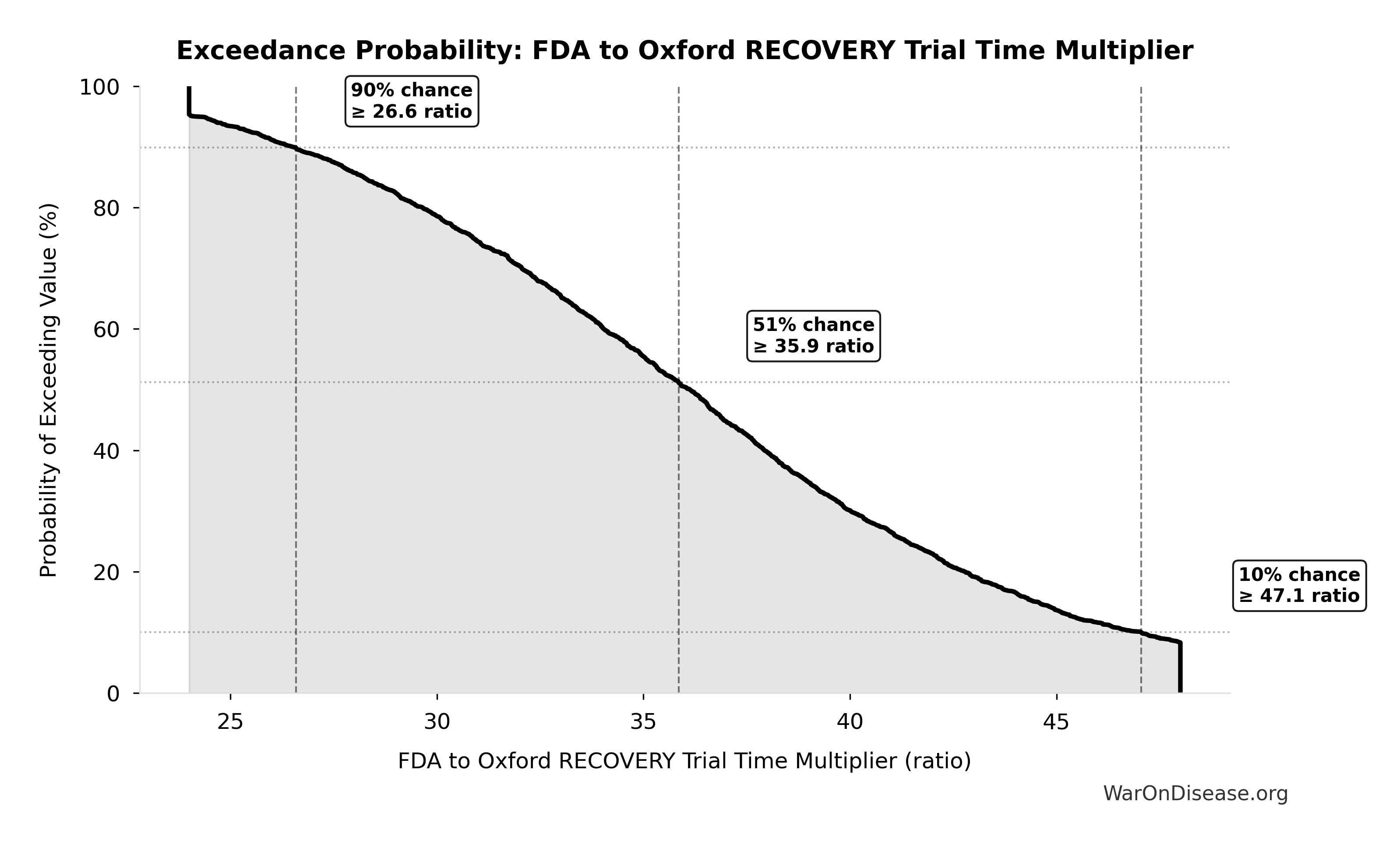
Sensitivity Indices for Total Economic Benefit from Elimination of Efficacy Lag Plus Earlier Treatment Discovery from Higher Trial Throughput
Regression-based sensitivity showing which inputs explain the most variance in the output.
| Input Parameter | Sensitivity Coefficient | Interpretation |
|---|---|---|
| Total DALYs from Elimination of Efficacy Lag Plus Earlier Treatment Discovery from Higher Trial Throughput (DALYs) | 1.7788 | Strong driver |
| Standard Economic Value per QALY (USD/QALY) | 1.3381 | Strong driver |
Interpretation: Standardized coefficients show the change in output (in SD units) per 1 SD change in input. Values near ±1 indicate strong influence; values exceeding ±1 may occur with correlated inputs.
Monte Carlo Distribution
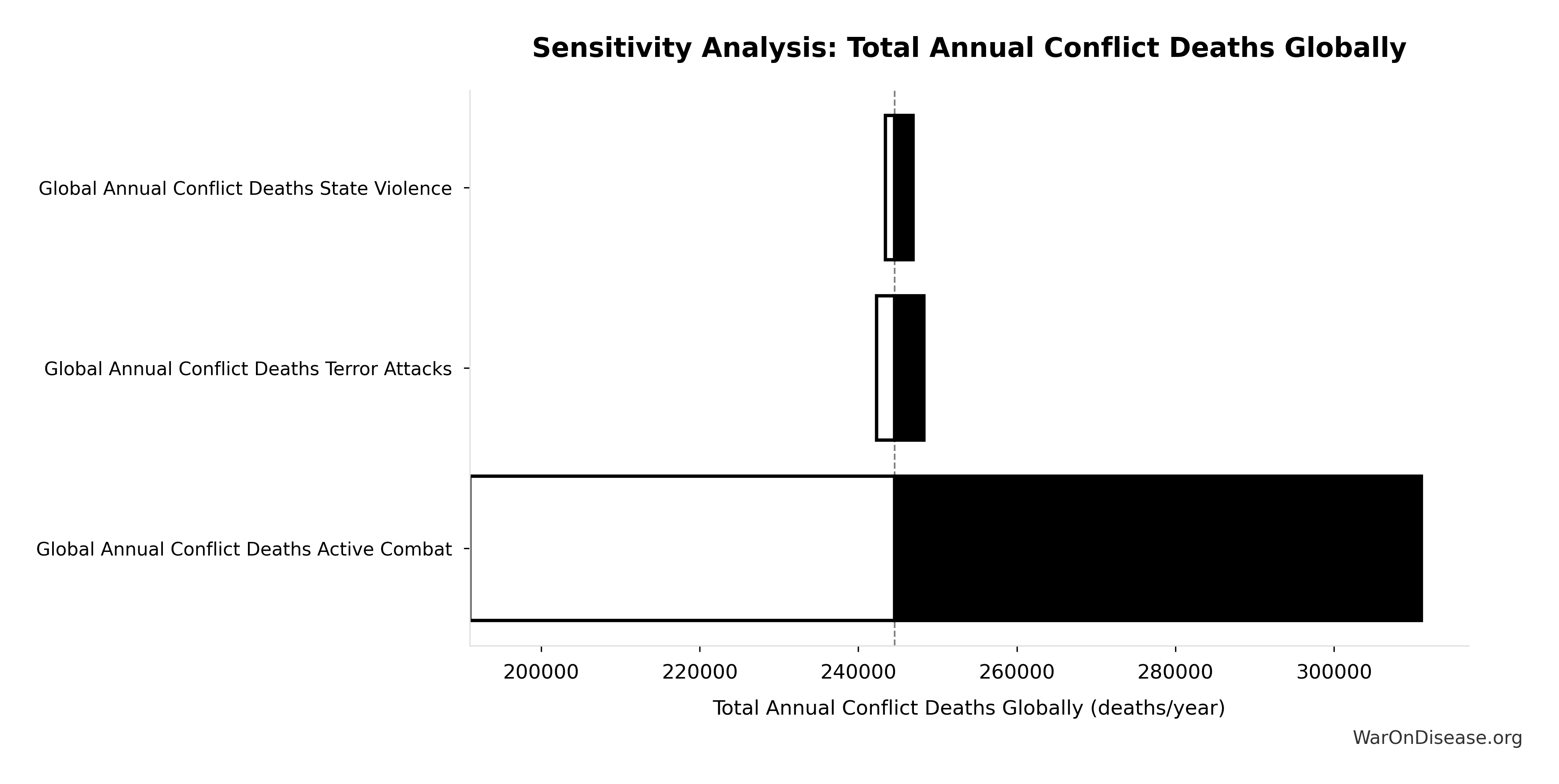
Simulation Results Summary: Total Economic Benefit from Elimination of Efficacy Lag Plus Earlier Treatment Discovery from Higher Trial Throughput
| Statistic | Value |
|---|---|
| Baseline (deterministic) | $84.8 quadrillion |
| Mean (expected value) | $87.8 quadrillion |
| Median (50th percentile) | $92.9 quadrillion |
| Standard Deviation | $11.5 quadrillion |
| 90% Range (5th-95th percentile) | [$62.4 quadrillion, $97.3 quadrillion] |
The histogram shows the distribution of Total Economic Benefit from Elimination of Efficacy Lag Plus Earlier Treatment Discovery from Higher Trial Throughput across 10,000 Monte Carlo simulations. The CDF (right) shows the probability of the outcome exceeding any given value, which is useful for risk assessment.
Exceedance Probability
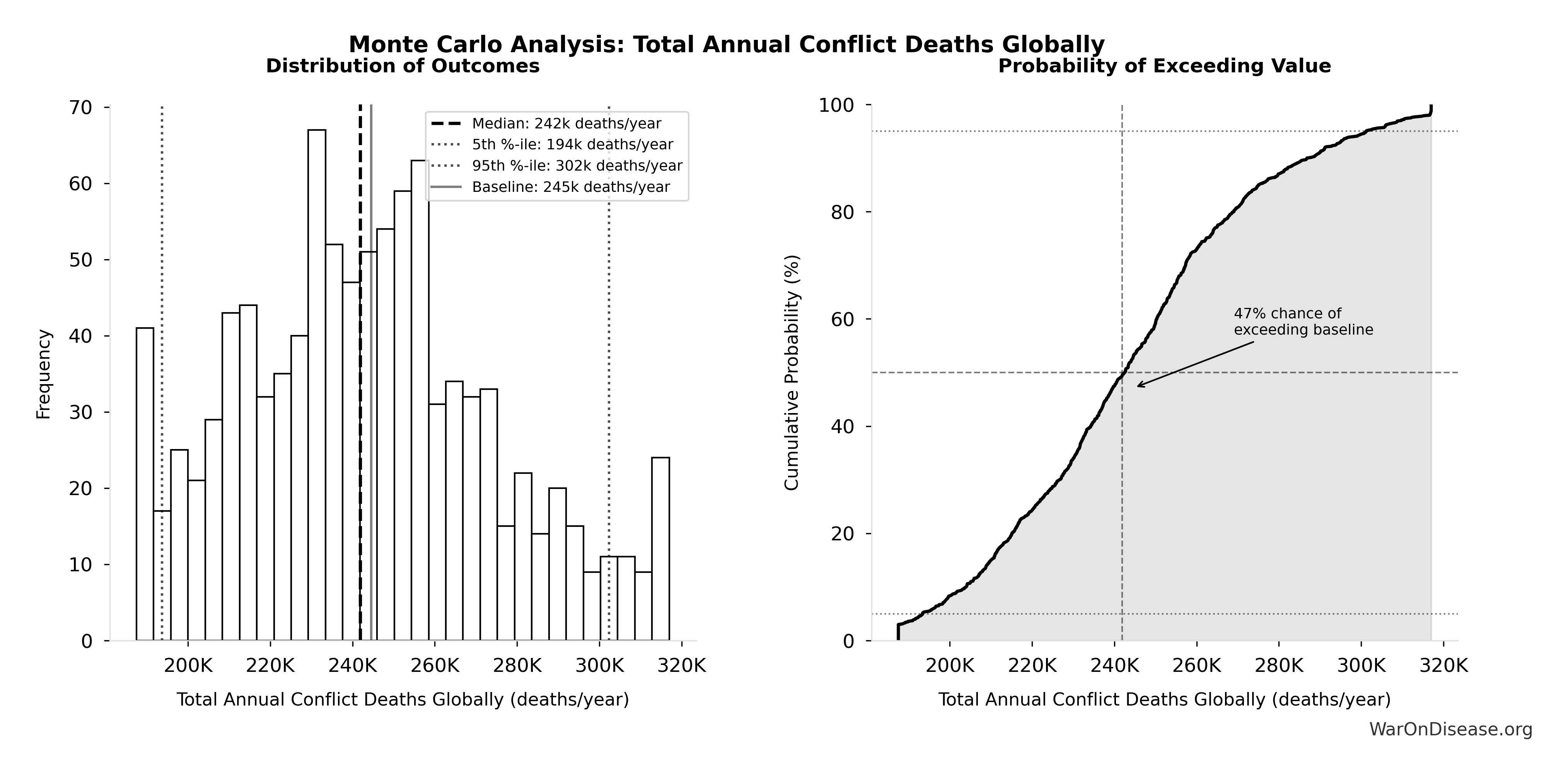
This exceedance probability chart shows the likelihood that Total Economic Benefit from Elimination of Efficacy Lag Plus Earlier Treatment Discovery from Higher Trial Throughput will exceed any given threshold. Higher curves indicate more favorable outcomes with greater certainty.
Total Lives Saved from Elimination of Efficacy Lag Plus Earlier Treatment Discovery from Higher Trial Throughput: 10.7 billion deaths
Note📊 Details
Total eventually avoidable deaths from the combined dFDA timeline shift. Represents deaths prevented when cures arrive earlier due to both increased trial capacity and eliminated efficacy lag.
Inputs:
- Global Daily Deaths from Disease and Aging 📊: 150 thousand deaths/day (SE: ±7.5 thousand deaths/day)
- dFDA Average Total Timeline Shift 🔢: 212 years
\[ \begin{gathered} Lives_{max} \\ = Deaths_{disease,daily} \times T_{accel,max} \times 338 \\ = 150{,}000 \times 212 \times 338 \\ = 10.7B \end{gathered} \] where: \[ T_{accel,max} = T_{accel} + T_{lag} = 204 + 8.2 = 212 \] where: \[ \begin{gathered} T_{accel} \\ = T_{first,SQ} \times \left(1 - \frac{1}{k_{capacity}}\right) \\ = 222 \times \left(1 - \frac{1}{12.3}\right) \\ = 204 \end{gathered} \] where: \[ \begin{gathered} T_{first,SQ} \\ = T_{queue,SQ} \times 0.5 \\ = 443 \times 0.5 \\ = 222 \end{gathered} \] where: \[ \begin{gathered} T_{queue,SQ} \\ = \frac{N_{untreated}}{Treatments_{new,ann}} \\ = \frac{6{,}650}{15} \\ = 443 \end{gathered} \] where: \[ \begin{gathered} N_{untreated} \\ = N_{rare} \times 0.95 \\ = 7{,}000 \times 0.95 \\ = 6{,}650 \end{gathered} \] where: \[ \begin{gathered} k_{capacity} \\ = \frac{N_{fundable,dFDA}}{Slots_{curr}} \\ = \frac{23.4M}{1.9M} \\ = 12.3 \end{gathered} \] where: \[ \begin{gathered} N_{fundable,dFDA} \\ = \frac{Subsidies_{dFDA,ann}}{Cost_{pragmatic,pt}} \\ = \frac{\$21.8B}{\$929} \\ = 23.4M \end{gathered} \] where: \[ \begin{gathered} Subsidies_{dFDA,ann} \\ = Funding_{dFDA,ann} - OPEX_{dFDA} \\ = \$21.8B - \$40M \\ = \$21.8B \end{gathered} \] where: \[ \begin{gathered} OPEX_{dFDA} \\ = Cost_{platform} + Cost_{staff} + Cost_{infra} \\ + Cost_{regulatory} + Cost_{community} \\ = \$15M + \$10M + \$8M + \$5M + \$2M \\ = \$40M \end{gathered} \] ? Low confidence
Sensitivity Analysis
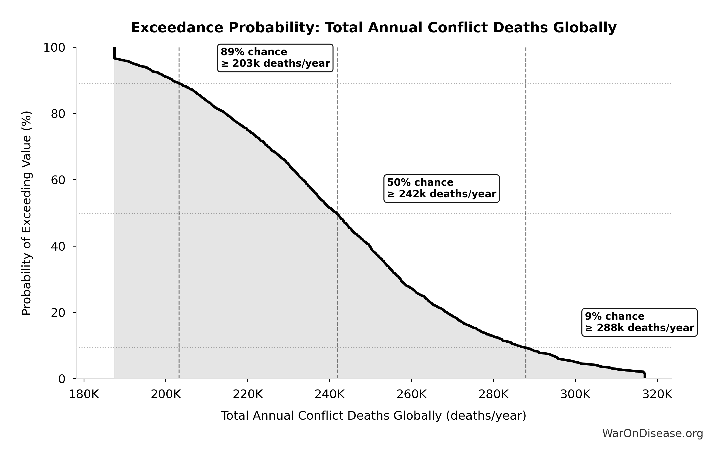
Sensitivity Indices for Total Lives Saved from Elimination of Efficacy Lag Plus Earlier Treatment Discovery from Higher Trial Throughput
Regression-based sensitivity showing which inputs explain the most variance in the output.
| Input Parameter | Sensitivity Coefficient | Interpretation |
|---|---|---|
| dFDA Average Total Timeline Shift (years) | 1.0374 | Strong driver |
| Global Daily Deaths from Disease and Aging (deaths/day) | 0.0406 | Minimal effect |
Interpretation: Standardized coefficients show the change in output (in SD units) per 1 SD change in input. Values near ±1 indicate strong influence; values exceeding ±1 may occur with correlated inputs.
Monte Carlo Distribution
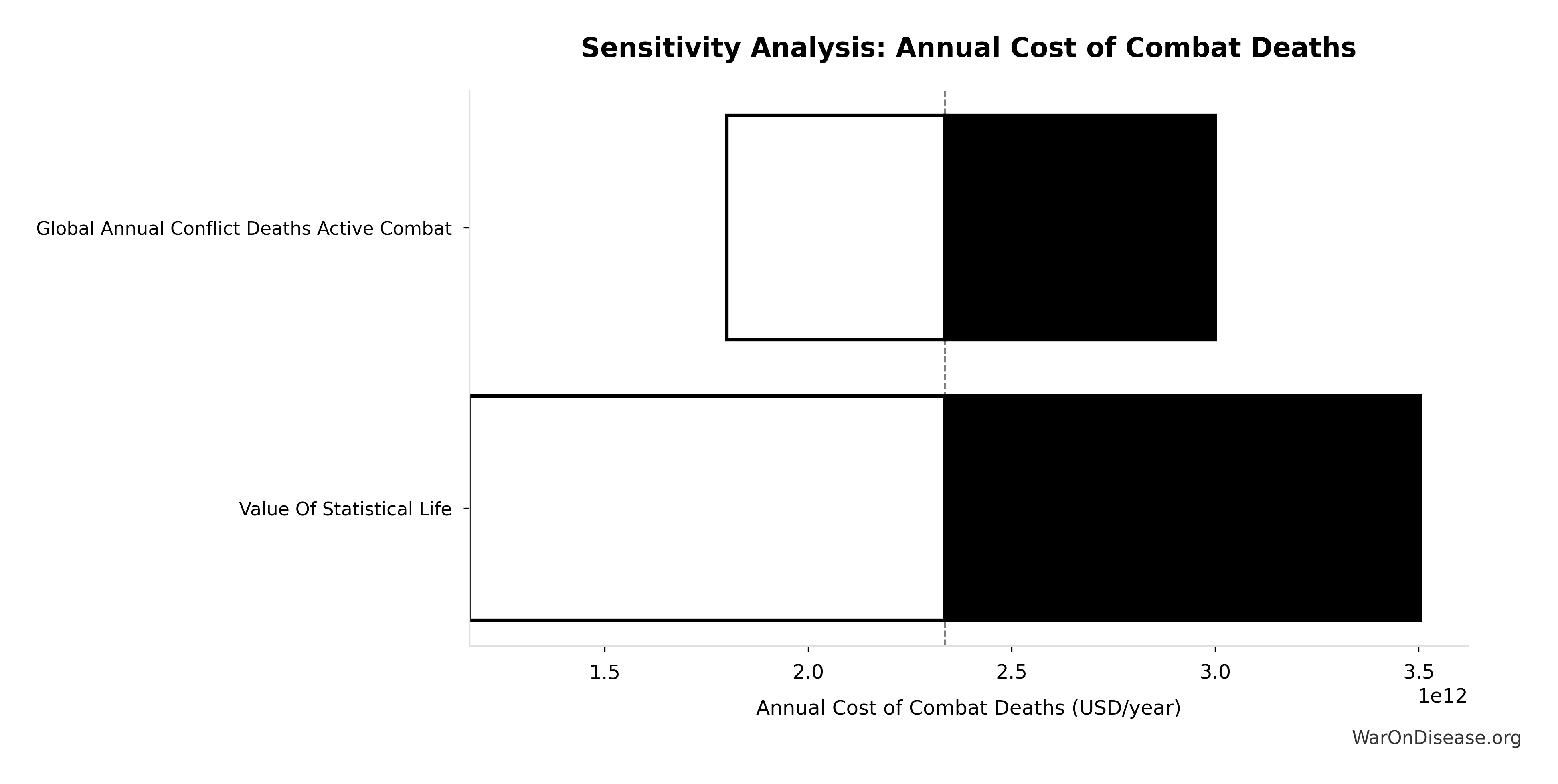
Simulation Results Summary: Total Lives Saved from Elimination of Efficacy Lag Plus Earlier Treatment Discovery from Higher Trial Throughput
| Statistic | Value |
|---|---|
| Baseline (deterministic) | 10.7 billion |
| Mean (expected value) | 11.7 billion |
| Median (50th percentile) | 11.7 billion |
| Standard Deviation | 2.45 billion |
| 90% Range (5th-95th percentile) | [7.4 billion, 16.2 billion] |
The histogram shows the distribution of Total Lives Saved from Elimination of Efficacy Lag Plus Earlier Treatment Discovery from Higher Trial Throughput across 10,000 Monte Carlo simulations. The CDF (right) shows the probability of the outcome exceeding any given value, which is useful for risk assessment.
Exceedance Probability
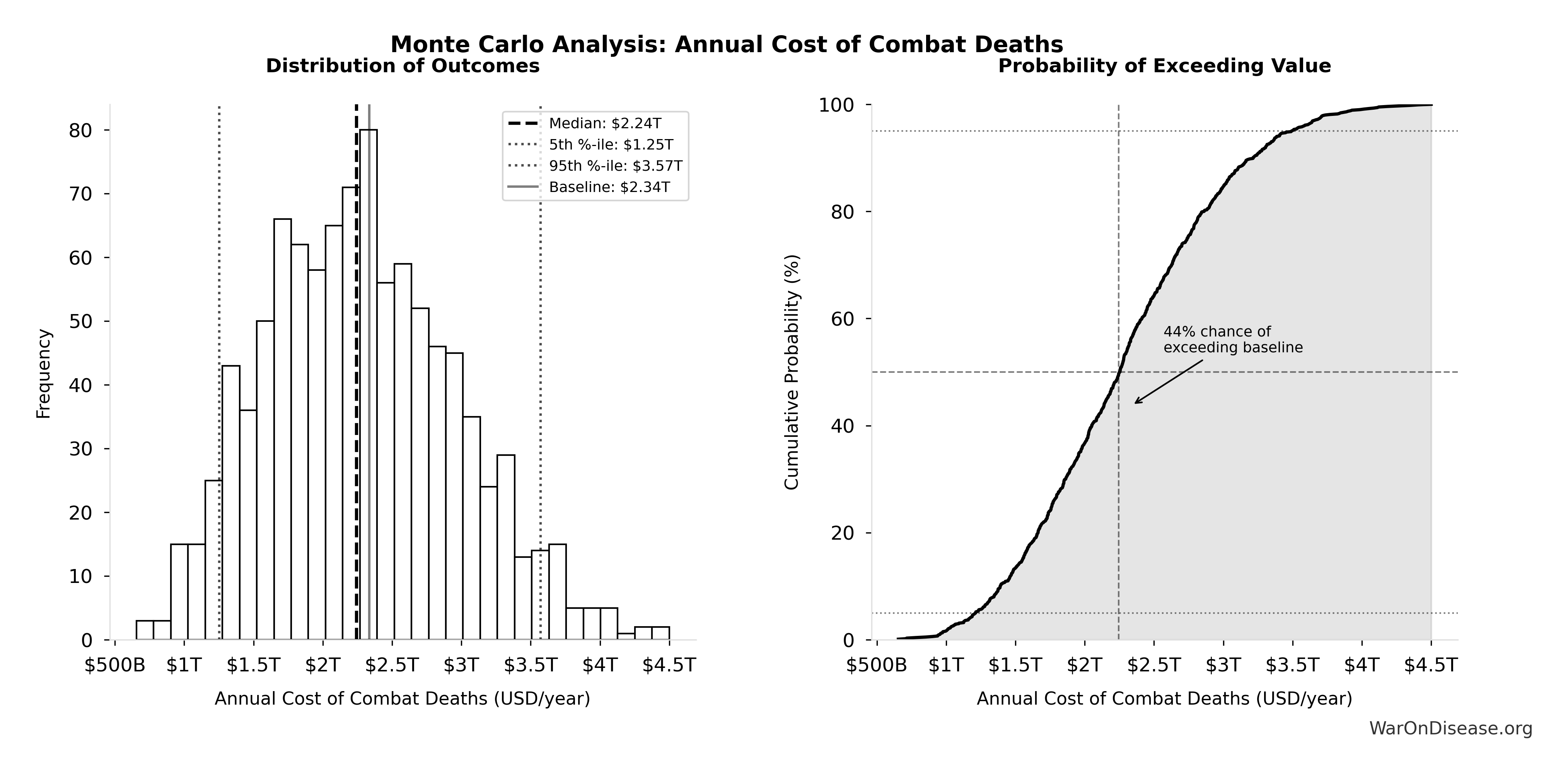
This exceedance probability chart shows the likelihood that Total Lives Saved from Elimination of Efficacy Lag Plus Earlier Treatment Discovery from Higher Trial Throughput will exceed any given threshold. Higher curves indicate more favorable outcomes with greater certainty.
Suffering Hours Eliminated from Elimination of Efficacy Lag Plus Earlier Treatment Discovery from Higher Trial Throughput: 1.93 quadrillion hours
Note📊 Details
Hours of suffering eliminated from the combined dFDA timeline shift. Calculated from YLD component of DALYs (39% of total DALYs × hours per year). One-time benefit, not annual recurring.
Inputs:
- Total DALYs from Elimination of Efficacy Lag Plus Earlier Treatment Discovery from Higher Trial Throughput 🔢: 565 billion DALYs
- YLD Proportion of Total DALYs 📊: 0.39 proportion (SE: ±0.03 proportion)
\[ \begin{gathered} Hours_{suffer,max} \\ = DALYs_{max} \times Pct_{YLD} \times 8760 \\ = 565B \times 0.39 \times 8760 \\ = 1930T \end{gathered} \] where: \[ \begin{gathered} DALYs_{max} \\ = DALYs_{global,ann} \times Pct_{avoid,DALY} \times T_{accel,max} \\ = 2.88B \times 92.6\% \times 212 \\ = 565B \end{gathered} \] where: \[ T_{accel,max} = T_{accel} + T_{lag} = 204 + 8.2 = 212 \] where: \[ \begin{gathered} T_{accel} \\ = T_{first,SQ} \times \left(1 - \frac{1}{k_{capacity}}\right) \\ = 222 \times \left(1 - \frac{1}{12.3}\right) \\ = 204 \end{gathered} \] where: \[ \begin{gathered} T_{first,SQ} \\ = T_{queue,SQ} \times 0.5 \\ = 443 \times 0.5 \\ = 222 \end{gathered} \] where: \[ \begin{gathered} T_{queue,SQ} \\ = \frac{N_{untreated}}{Treatments_{new,ann}} \\ = \frac{6{,}650}{15} \\ = 443 \end{gathered} \] where: \[ \begin{gathered} N_{untreated} \\ = N_{rare} \times 0.95 \\ = 7{,}000 \times 0.95 \\ = 6{,}650 \end{gathered} \] where: \[ \begin{gathered} k_{capacity} \\ = \frac{N_{fundable,dFDA}}{Slots_{curr}} \\ = \frac{23.4M}{1.9M} \\ = 12.3 \end{gathered} \] where: \[ \begin{gathered} N_{fundable,dFDA} \\ = \frac{Subsidies_{dFDA,ann}}{Cost_{pragmatic,pt}} \\ = \frac{\$21.8B}{\$929} \\ = 23.4M \end{gathered} \] where: \[ \begin{gathered} Subsidies_{dFDA,ann} \\ = Funding_{dFDA,ann} - OPEX_{dFDA} \\ = \$21.8B - \$40M \\ = \$21.8B \end{gathered} \] where: \[ \begin{gathered} OPEX_{dFDA} \\ = Cost_{platform} + Cost_{staff} + Cost_{infra} \\ + Cost_{regulatory} + Cost_{community} \\ = \$15M + \$10M + \$8M + \$5M + \$2M \\ = \$40M \end{gathered} \] ? Low confidence
Sensitivity Analysis
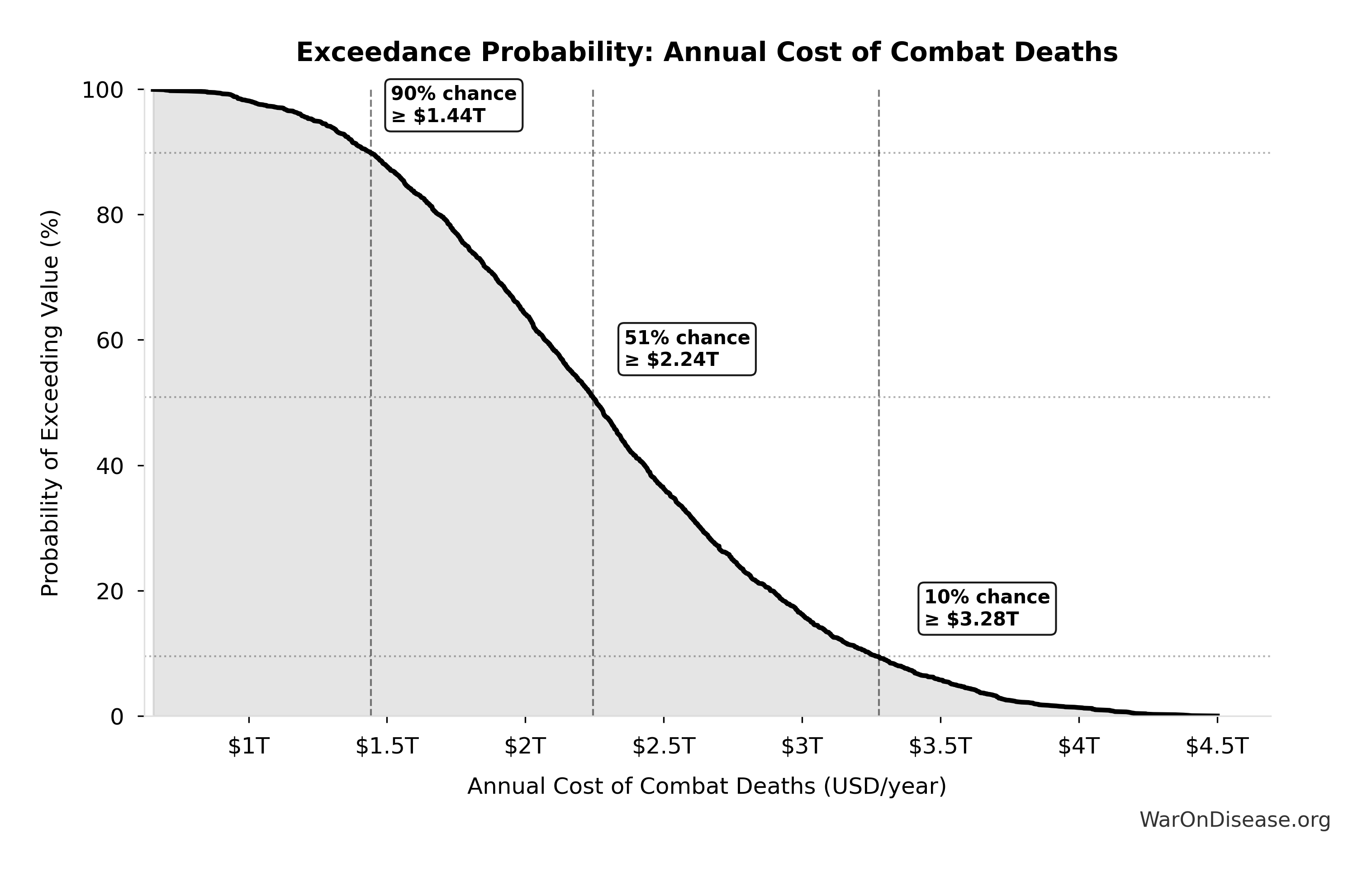
Sensitivity Indices for Suffering Hours Eliminated from Elimination of Efficacy Lag Plus Earlier Treatment Discovery from Higher Trial Throughput
Regression-based sensitivity showing which inputs explain the most variance in the output.
| Input Parameter | Sensitivity Coefficient | Interpretation |
|---|---|---|
| Total DALYs from Elimination of Efficacy Lag Plus Earlier Treatment Discovery from Higher Trial Throughput (DALYs) | 1.3102 | Strong driver |
| YLD Proportion of Total DALYs (proportion) | 0.3977 | Moderate driver |
Interpretation: Standardized coefficients show the change in output (in SD units) per 1 SD change in input. Values near ±1 indicate strong influence; values exceeding ±1 may occur with correlated inputs.
Monte Carlo Distribution
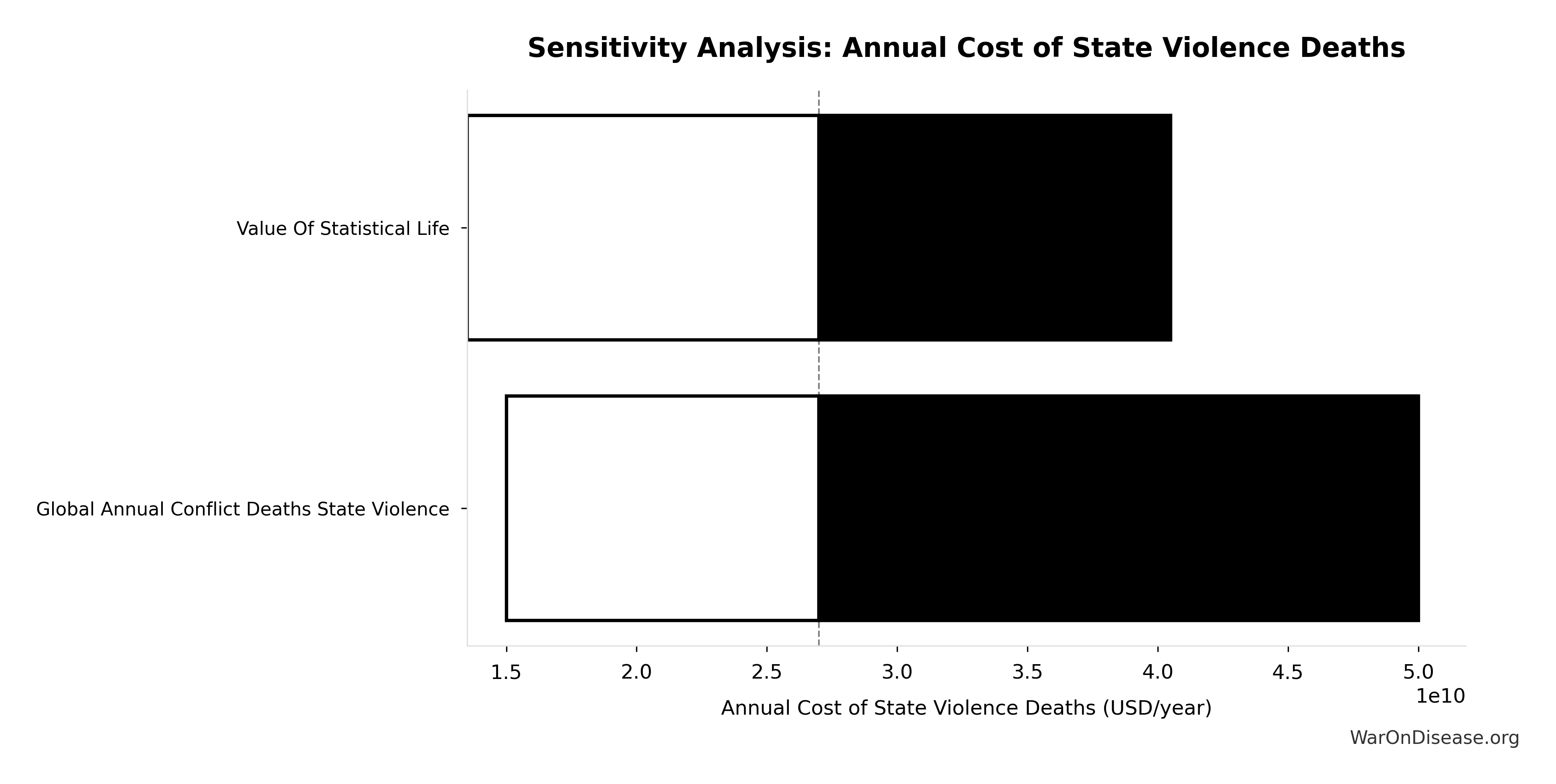
Simulation Results Summary: Suffering Hours Eliminated from Elimination of Efficacy Lag Plus Earlier Treatment Discovery from Higher Trial Throughput
| Statistic | Value |
|---|---|
| Baseline (deterministic) | 1.93 quadrillion |
| Mean (expected value) | 2.05 quadrillion |
| Median (50th percentile) | 2.11 quadrillion |
| Standard Deviation | 374 trillion |
| 90% Range (5th-95th percentile) | [1.36 quadrillion, 2.62 quadrillion] |
The histogram shows the distribution of Suffering Hours Eliminated from Elimination of Efficacy Lag Plus Earlier Treatment Discovery from Higher Trial Throughput across 10,000 Monte Carlo simulations. The CDF (right) shows the probability of the outcome exceeding any given value, which is useful for risk assessment.
Exceedance Probability
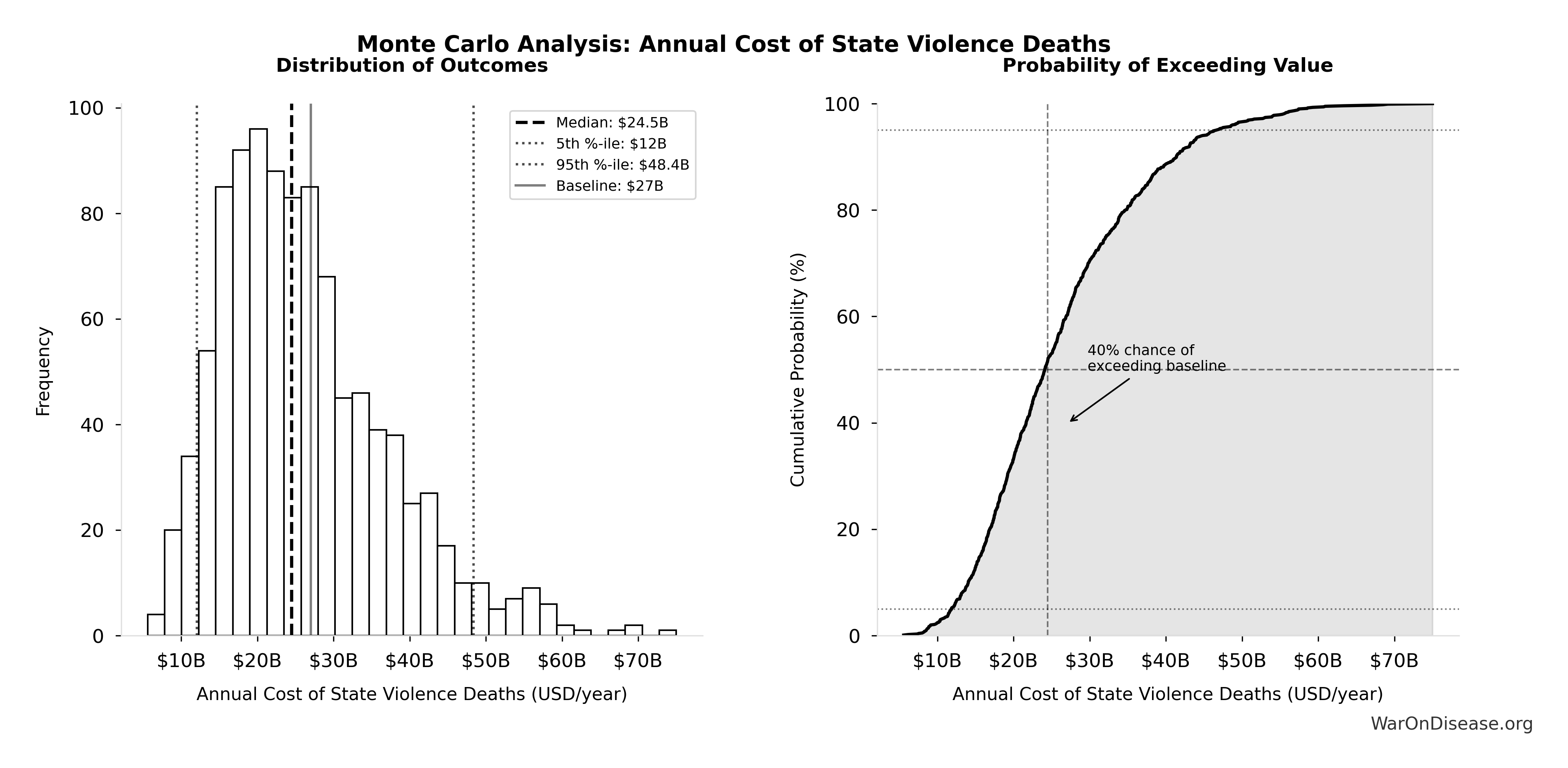
This exceedance probability chart shows the likelihood that Suffering Hours Eliminated from Elimination of Efficacy Lag Plus Earlier Treatment Discovery from Higher Trial Throughput will exceed any given threshold. Higher curves indicate more favorable outcomes with greater certainty.
dFDA Average Total Timeline Shift: 212 years
Note📊 Details
Average years earlier patients receive treatments due to dFDA. Combines treatment timeline acceleration from increased trial capacity with efficacy lag elimination for treatments already discovered.
Inputs:
- dFDA Treatment Timeline Acceleration 🔢: 204 years
- Regulatory Delay for Efficacy Testing Post-Safety Verification 📊: 8.2 years (SE: ±2 years)
\[ T_{accel,max} = T_{accel} + T_{lag} = 204 + 8.2 = 212 \] where: \[ \begin{gathered} T_{accel} \\ = T_{first,SQ} \times \left(1 - \frac{1}{k_{capacity}}\right) \\ = 222 \times \left(1 - \frac{1}{12.3}\right) \\ = 204 \end{gathered} \] where: \[ \begin{gathered} T_{first,SQ} \\ = T_{queue,SQ} \times 0.5 \\ = 443 \times 0.5 \\ = 222 \end{gathered} \] where: \[ \begin{gathered} T_{queue,SQ} \\ = \frac{N_{untreated}}{Treatments_{new,ann}} \\ = \frac{6{,}650}{15} \\ = 443 \end{gathered} \] where: \[ \begin{gathered} N_{untreated} \\ = N_{rare} \times 0.95 \\ = 7{,}000 \times 0.95 \\ = 6{,}650 \end{gathered} \] where: \[ \begin{gathered} k_{capacity} \\ = \frac{N_{fundable,dFDA}}{Slots_{curr}} \\ = \frac{23.4M}{1.9M} \\ = 12.3 \end{gathered} \] where: \[ \begin{gathered} N_{fundable,dFDA} \\ = \frac{Subsidies_{dFDA,ann}}{Cost_{pragmatic,pt}} \\ = \frac{\$21.8B}{\$929} \\ = 23.4M \end{gathered} \] where: \[ \begin{gathered} Subsidies_{dFDA,ann} \\ = Funding_{dFDA,ann} - OPEX_{dFDA} \\ = \$21.8B - \$40M \\ = \$21.8B \end{gathered} \] where: \[ \begin{gathered} OPEX_{dFDA} \\ = Cost_{platform} + Cost_{staff} + Cost_{infra} \\ + Cost_{regulatory} + Cost_{community} \\ = \$15M + \$10M + \$8M + \$5M + \$2M \\ = \$40M \end{gathered} \] ? Low confidence
Sensitivity Analysis
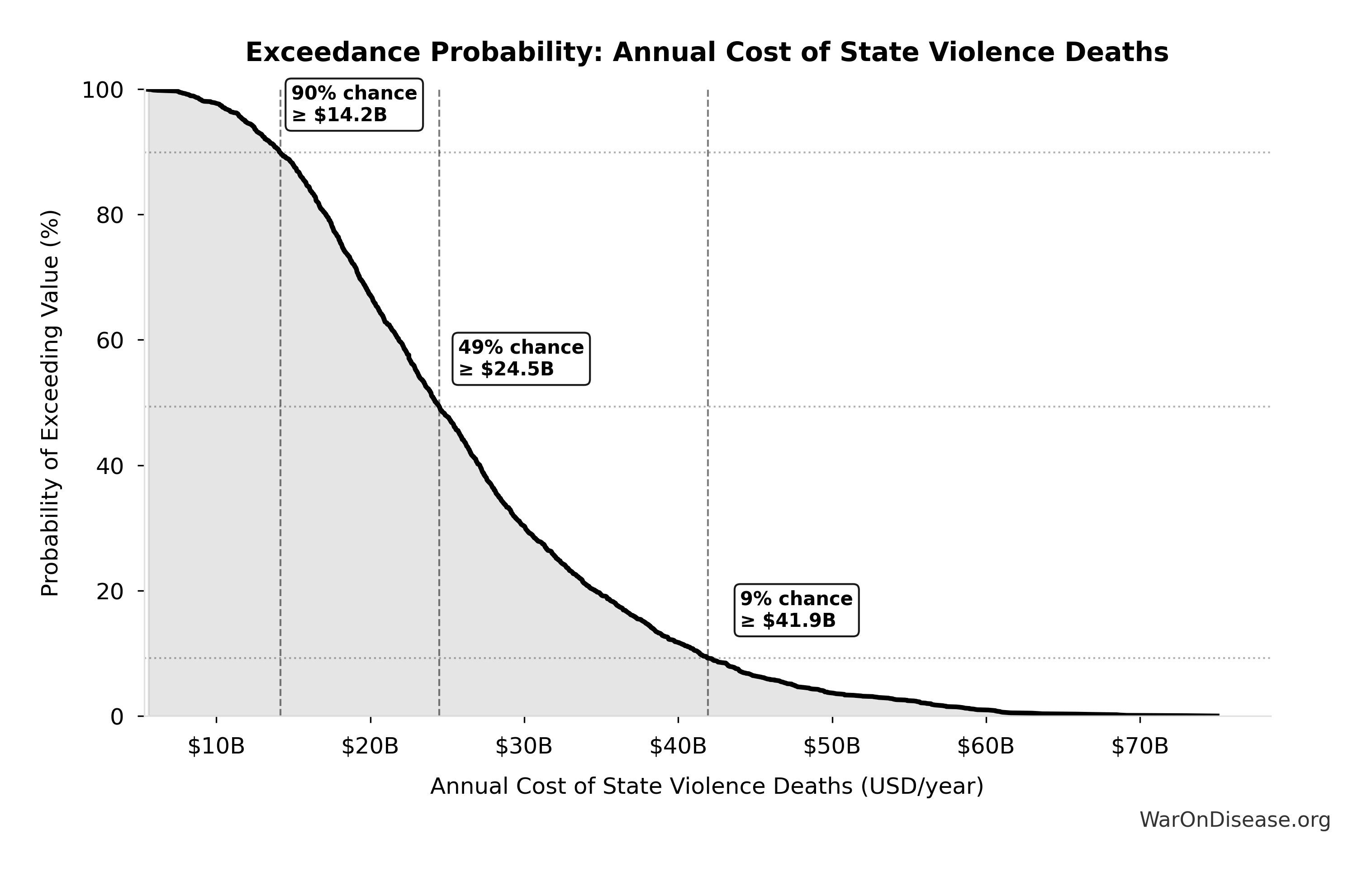
Sensitivity Indices for dFDA Average Total Timeline Shift
Regression-based sensitivity showing which inputs explain the most variance in the output.
| Input Parameter | Sensitivity Coefficient | Interpretation |
|---|---|---|
| dFDA Treatment Timeline Acceleration (years) | 1.0325 | Strong driver |
| Regulatory Delay for Efficacy Testing Post-Safety Verification (years) | 0.0328 | Minimal effect |
Interpretation: Standardized coefficients show the change in output (in SD units) per 1 SD change in input. Values near ±1 indicate strong influence; values exceeding ±1 may occur with correlated inputs.
Monte Carlo Distribution
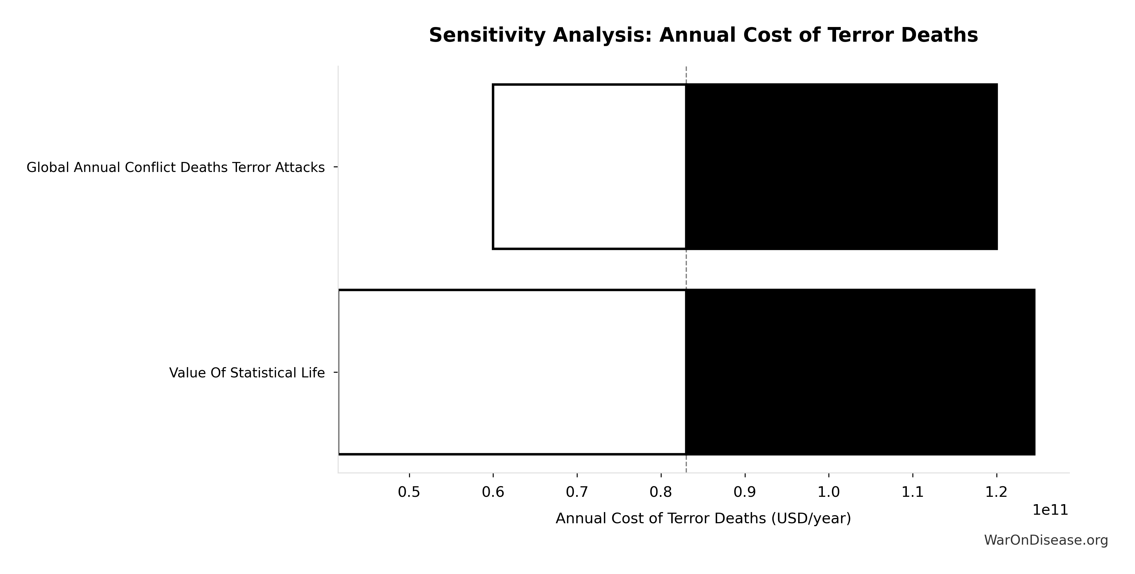
Simulation Results Summary: dFDA Average Total Timeline Shift
| Statistic | Value |
|---|---|
| Baseline (deterministic) | 212 |
| Mean (expected value) | 233 |
| Median (50th percentile) | 231 |
| Standard Deviation | 60.3 |
| 90% Range (5th-95th percentile) | [135, 355] |
The histogram shows the distribution of dFDA Average Total Timeline Shift across 10,000 Monte Carlo simulations. The CDF (right) shows the probability of the outcome exceeding any given value, which is useful for risk assessment.
Exceedance Probability
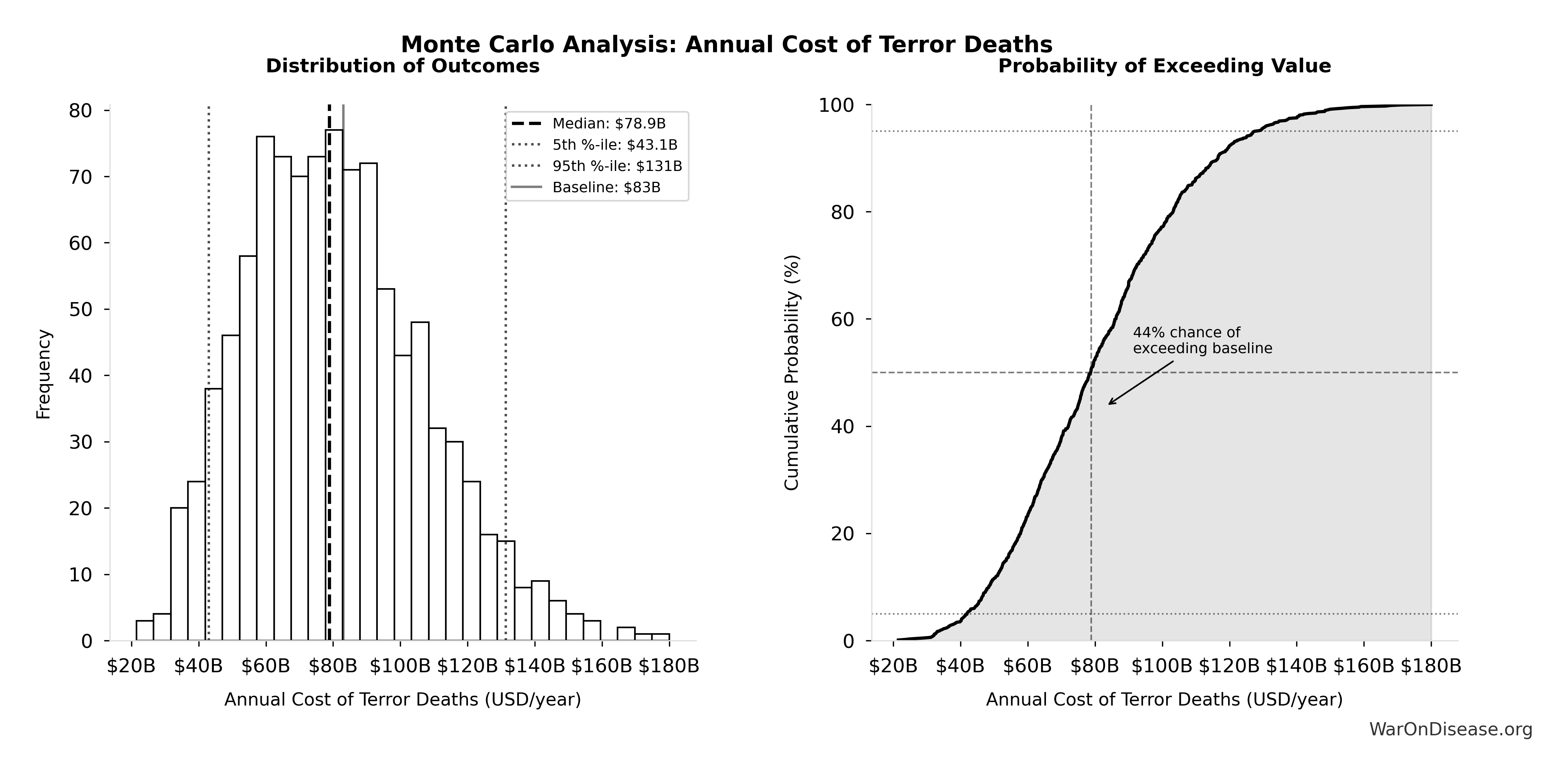
This exceedance probability chart shows the likelihood that dFDA Average Total Timeline Shift will exceed any given threshold. Higher curves indicate more favorable outcomes with greater certainty.
dFDA Treatment Timeline Acceleration: 204 years
Note📊 Details
Years earlier the average first treatment arrives due to dFDA’s trial capacity increase. Calculated as the status quo timeline reduced by the inverse of the capacity multiplier. Uses only trial capacity multiplier (not combined with valley of death rescue) because additional candidates don’t directly speed therapeutic space exploration.
Inputs:
- Status Quo Average Years to First Treatment 🔢: 222 years
- Trial Capacity Multiplier 🔢: 12.3x
\[ \begin{gathered} T_{accel} \\ = T_{first,SQ} \times \left(1 - \frac{1}{k_{capacity}}\right) \\ = 222 \times \left(1 - \frac{1}{12.3}\right) \\ = 204 \end{gathered} \] where: \[ \begin{gathered} T_{first,SQ} \\ = T_{queue,SQ} \times 0.5 \\ = 443 \times 0.5 \\ = 222 \end{gathered} \] where: \[ \begin{gathered} T_{queue,SQ} \\ = \frac{N_{untreated}}{Treatments_{new,ann}} \\ = \frac{6{,}650}{15} \\ = 443 \end{gathered} \] where: \[ \begin{gathered} N_{untreated} \\ = N_{rare} \times 0.95 \\ = 7{,}000 \times 0.95 \\ = 6{,}650 \end{gathered} \] where: \[ \begin{gathered} k_{capacity} \\ = \frac{N_{fundable,dFDA}}{Slots_{curr}} \\ = \frac{23.4M}{1.9M} \\ = 12.3 \end{gathered} \] where: \[ \begin{gathered} N_{fundable,dFDA} \\ = \frac{Subsidies_{dFDA,ann}}{Cost_{pragmatic,pt}} \\ = \frac{\$21.8B}{\$929} \\ = 23.4M \end{gathered} \] where: \[ \begin{gathered} Subsidies_{dFDA,ann} \\ = Funding_{dFDA,ann} - OPEX_{dFDA} \\ = \$21.8B - \$40M \\ = \$21.8B \end{gathered} \] where: \[ \begin{gathered} OPEX_{dFDA} \\ = Cost_{platform} + Cost_{staff} + Cost_{infra} \\ + Cost_{regulatory} + Cost_{community} \\ = \$15M + \$10M + \$8M + \$5M + \$2M \\ = \$40M \end{gathered} \] ? Low confidence
Sensitivity Analysis
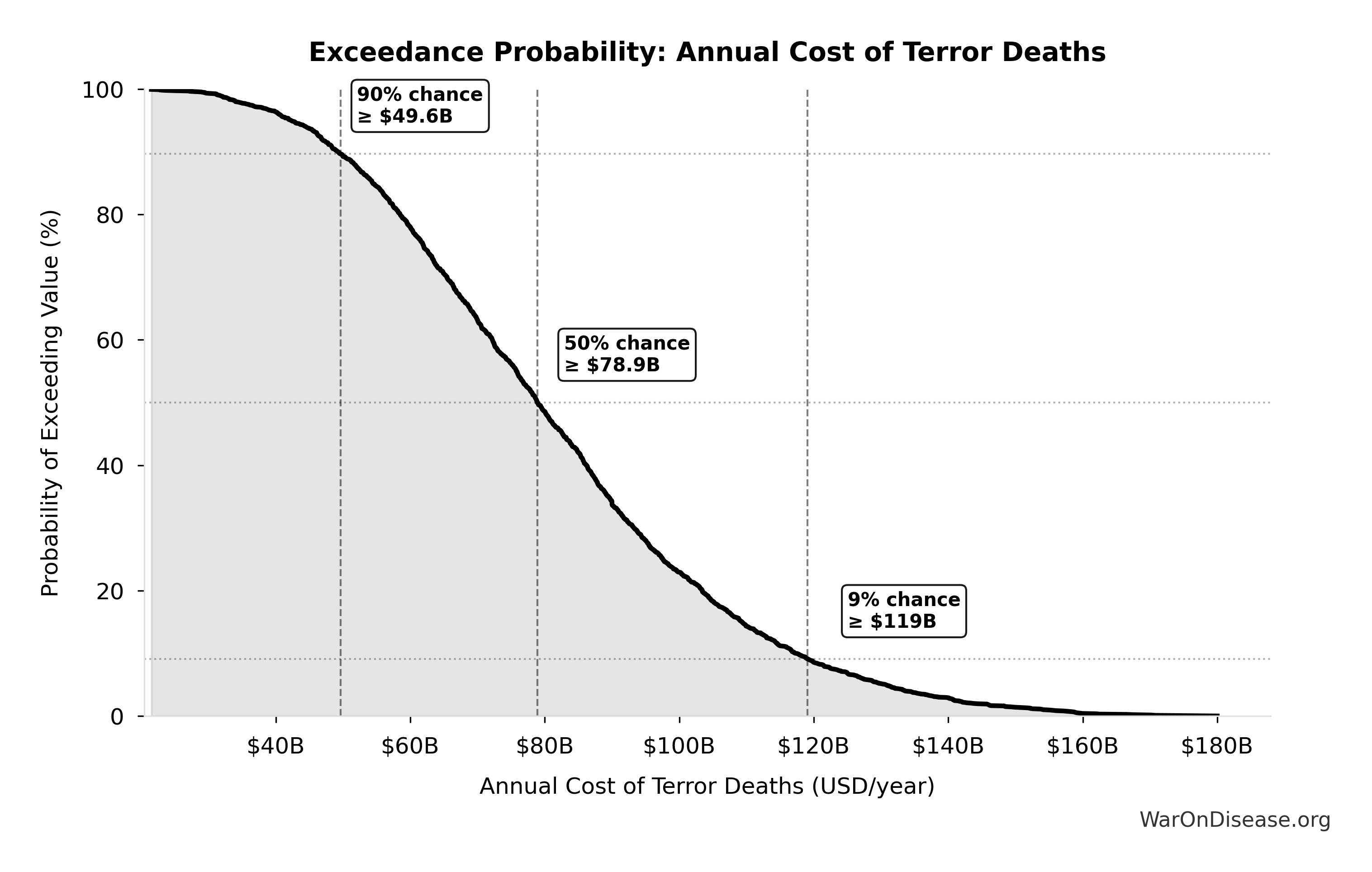
Sensitivity Indices for dFDA Treatment Timeline Acceleration
Regression-based sensitivity showing which inputs explain the most variance in the output.
| Input Parameter | Sensitivity Coefficient | Interpretation |
|---|---|---|
| Status Quo Average Years to First Treatment (years) | 1.0664 | Strong driver |
| Trial Capacity Multiplier (x) | -0.0777 | Minimal effect |
Interpretation: Standardized coefficients show the change in output (in SD units) per 1 SD change in input. Values near ±1 indicate strong influence; values exceeding ±1 may occur with correlated inputs.
Monte Carlo Distribution
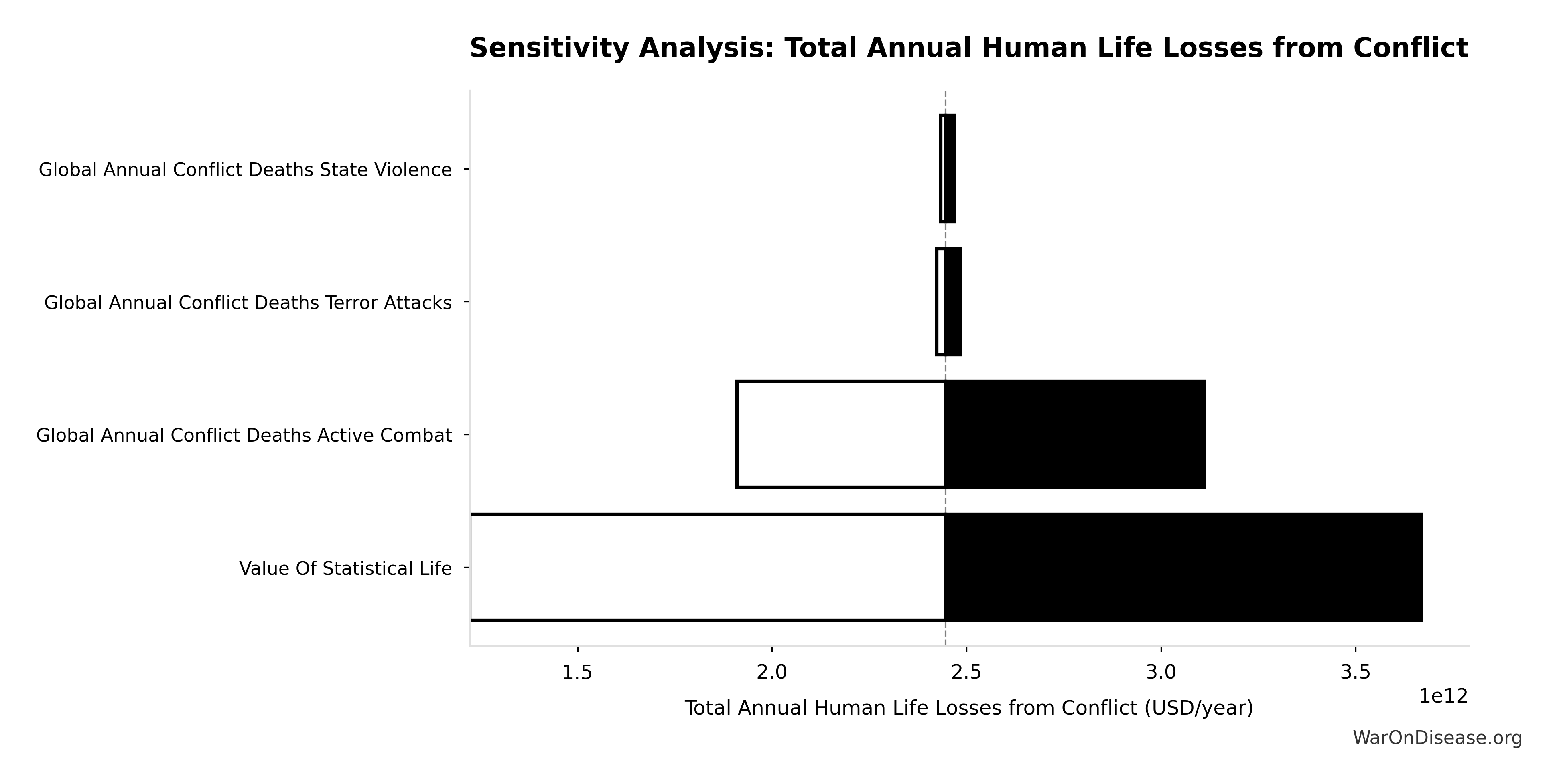
Simulation Results Summary: dFDA Treatment Timeline Acceleration
| Statistic | Value |
|---|---|
| Baseline (deterministic) | 204 |
| Mean (expected value) | 225 |
| Median (50th percentile) | 223 |
| Standard Deviation | 62.3 |
| 90% Range (5th-95th percentile) | [123, 350] |
The histogram shows the distribution of dFDA Treatment Timeline Acceleration across 10,000 Monte Carlo simulations. The CDF (right) shows the probability of the outcome exceeding any given value, which is useful for risk assessment.
Exceedance Probability
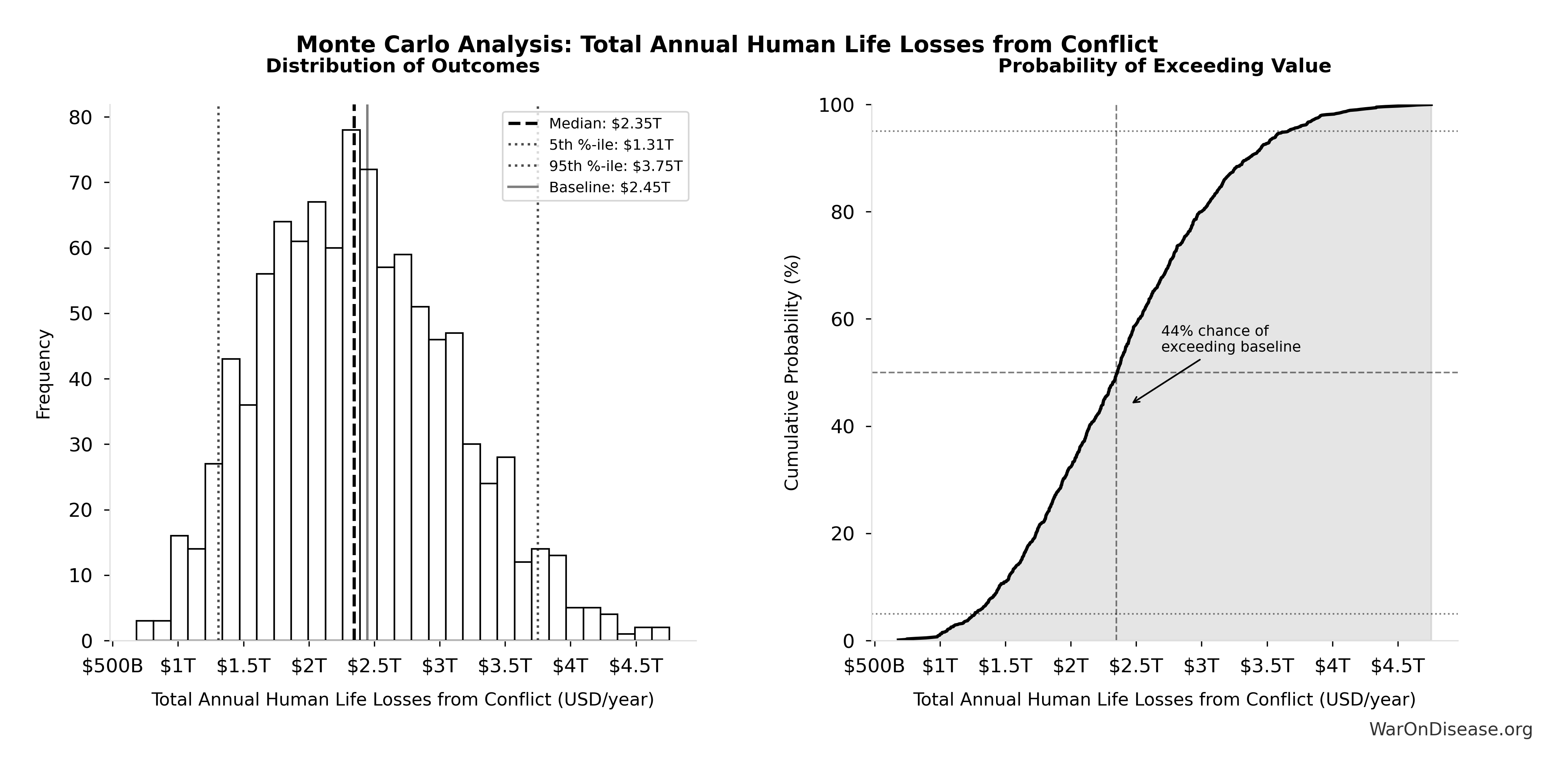
This exceedance probability chart shows the likelihood that dFDA Treatment Timeline Acceleration will exceed any given threshold. Higher curves indicate more favorable outcomes with greater certainty.
dFDA Trial Cost Reduction Factor: 44.1x
Note📊 Details
Cost reduction factor projected for dFDA pragmatic trials (traditional Phase 3 cost / dFDA pragmatic cost per patient)
Inputs:
- Phase 3 Cost per Patient 📊: $41K (95% CI: $20K - $120K)
- dFDA Pragmatic Trial Cost per Patient 📊: $929 (95% CI: $97 - $3K)
\[ \begin{gathered} k_{reduce} \\ = \frac{Cost_{P3,pt}}{Cost_{pragmatic,pt}} \\ = \frac{\$41K}{\$929} \\ = 44.1 \end{gathered} \]
✓ High confidence
Sensitivity Analysis
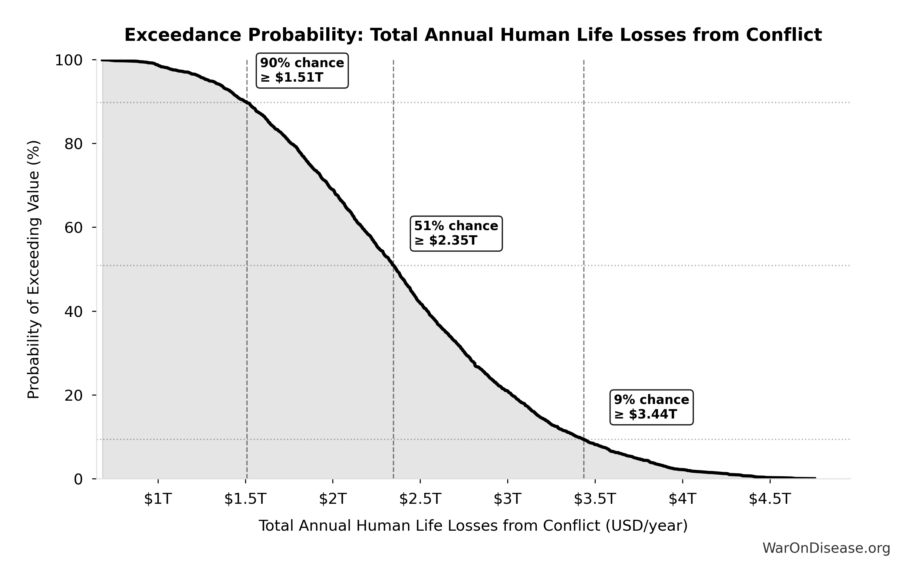
Sensitivity Indices for dFDA Trial Cost Reduction Factor
Regression-based sensitivity showing which inputs explain the most variance in the output.
| Input Parameter | Sensitivity Coefficient | Interpretation |
|---|---|---|
| dFDA Pragmatic Trial Cost per Patient (USD/patient) | -8.8326 | Strong driver |
| Phase 3 Cost per Patient (USD/patient) | 8.3341 | Strong driver |
Interpretation: Standardized coefficients show the change in output (in SD units) per 1 SD change in input. Values near ±1 indicate strong influence; values exceeding ±1 may occur with correlated inputs.
Monte Carlo Distribution
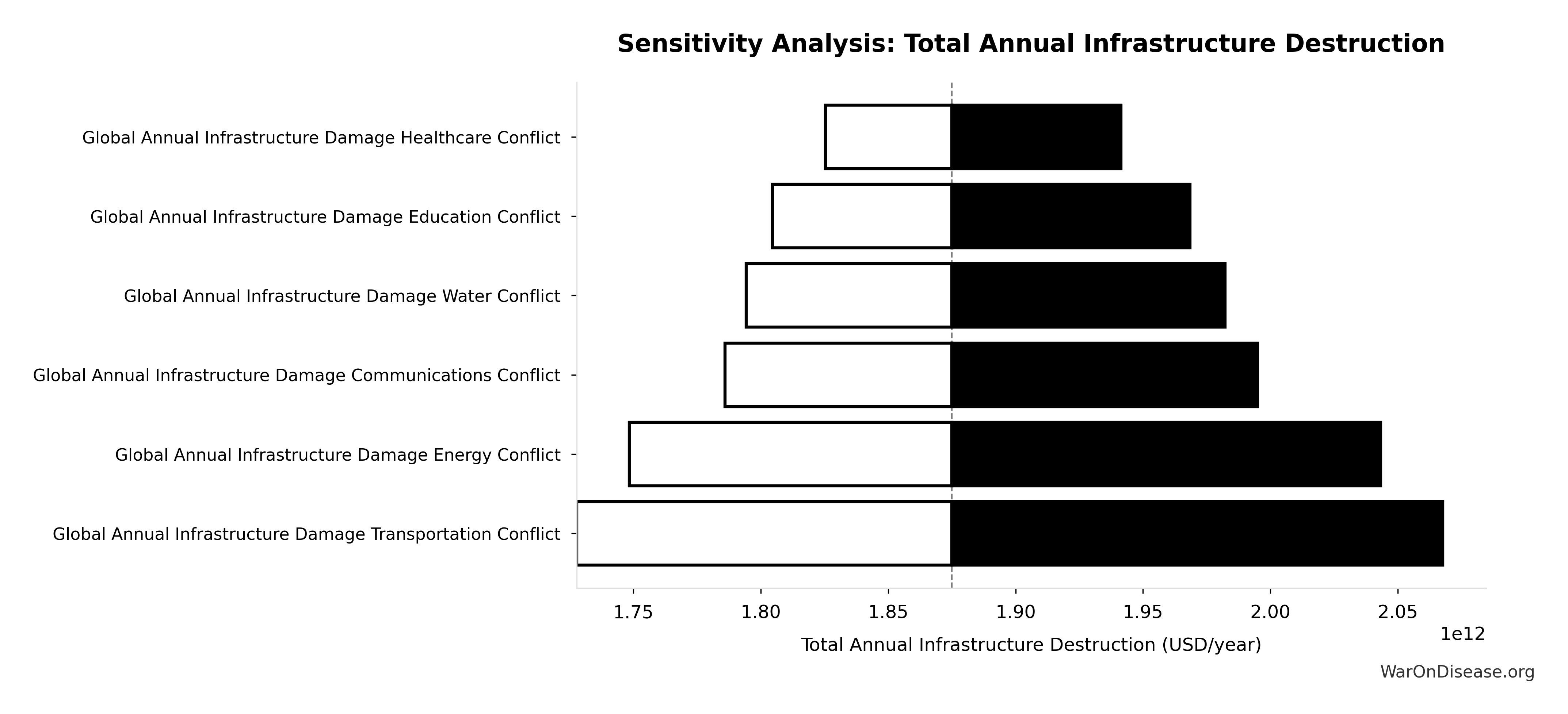
Simulation Results Summary: dFDA Trial Cost Reduction Factor
| Statistic | Value |
|---|---|
| Baseline (deterministic) | 44.1x |
| Mean (expected value) | 52.8x |
| Median (50th percentile) | 48x |
| Standard Deviation | 19.5x |
| 90% Range (5th-95th percentile) | [39.4x, 89.1x] |
The histogram shows the distribution of dFDA Trial Cost Reduction Factor across 10,000 Monte Carlo simulations. The CDF (right) shows the probability of the outcome exceeding any given value, which is useful for risk assessment.
Exceedance Probability
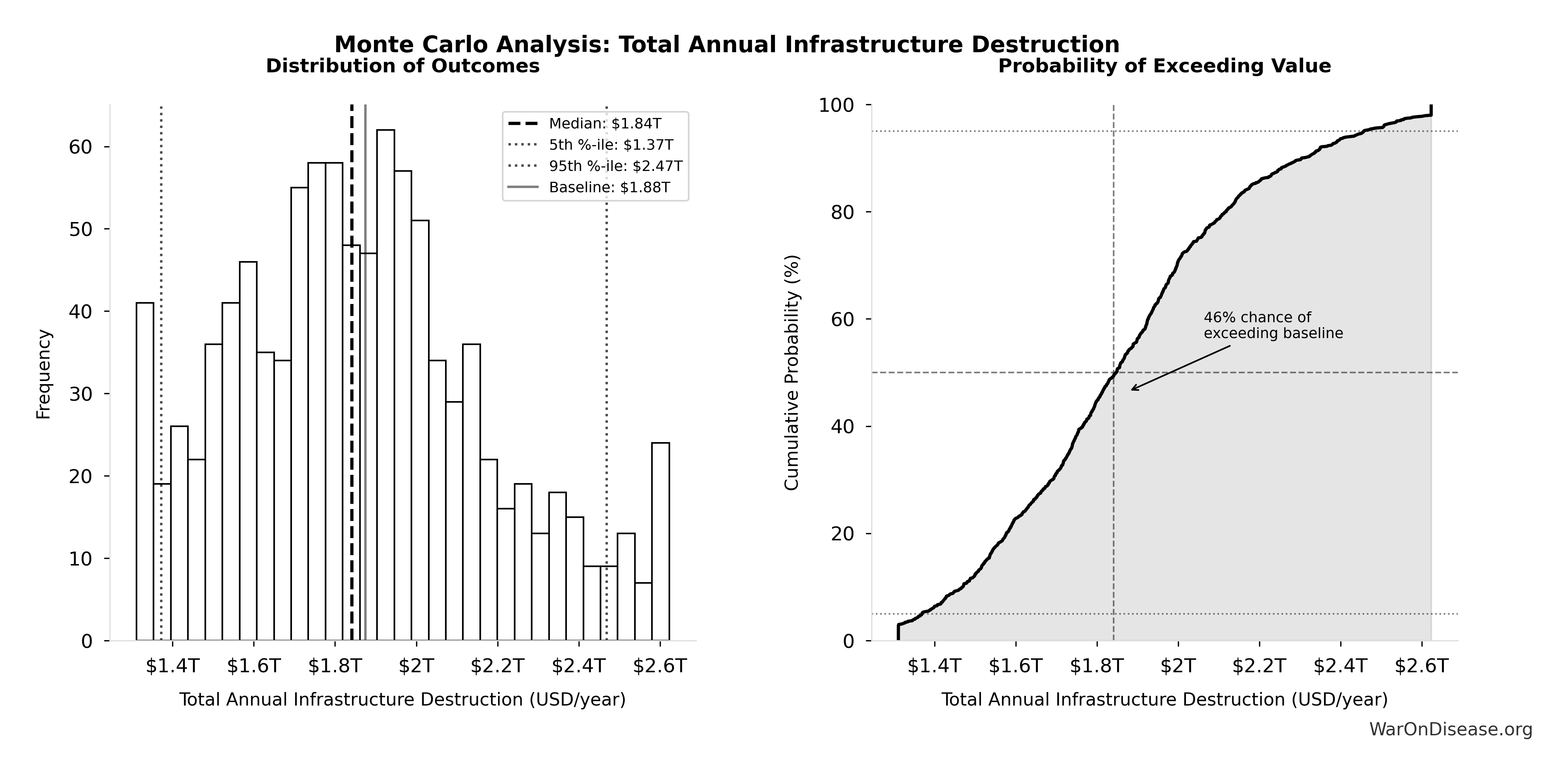
This exceedance probability chart shows the likelihood that dFDA Trial Cost Reduction Factor will exceed any given threshold. Higher curves indicate more favorable outcomes with greater certainty.
dFDA Trial Cost Reduction Percentage: 97.7%
Note📊 Details
Trial cost reduction percentage: 1 - (dFDA pragmatic cost / traditional Phase 3 cost)
Inputs:
- dFDA Pragmatic Trial Cost per Patient 📊: $929 (95% CI: $97 - $3K)
- Phase 3 Cost per Patient 📊: $41K (95% CI: $20K - $120K)
\[ \begin{gathered} Reduce_{pct} \\ = 1 - \frac{Cost_{pragmatic,pt}}{Cost_{P3,pt}} \\ = 1 - \frac{\$929}{\$41K} \\ = 97.7\% \end{gathered} \]
✓ High confidence
Sensitivity Analysis
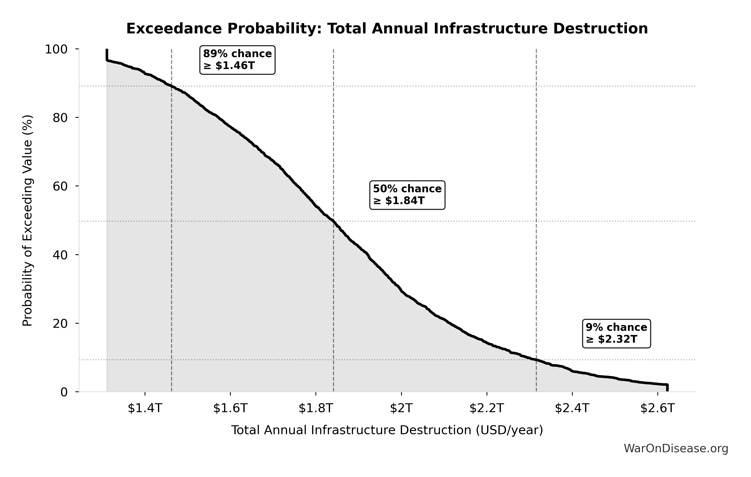
Sensitivity Indices for dFDA Trial Cost Reduction Percentage
Regression-based sensitivity showing which inputs explain the most variance in the output.
| Input Parameter | Sensitivity Coefficient | Interpretation |
|---|---|---|
| dFDA Pragmatic Trial Cost per Patient (USD/patient) | -6.4207 | Strong driver |
| Phase 3 Cost per Patient (USD/patient) | 5.6539 | Strong driver |
Interpretation: Standardized coefficients show the change in output (in SD units) per 1 SD change in input. Values near ±1 indicate strong influence; values exceeding ±1 may occur with correlated inputs.
Monte Carlo Distribution
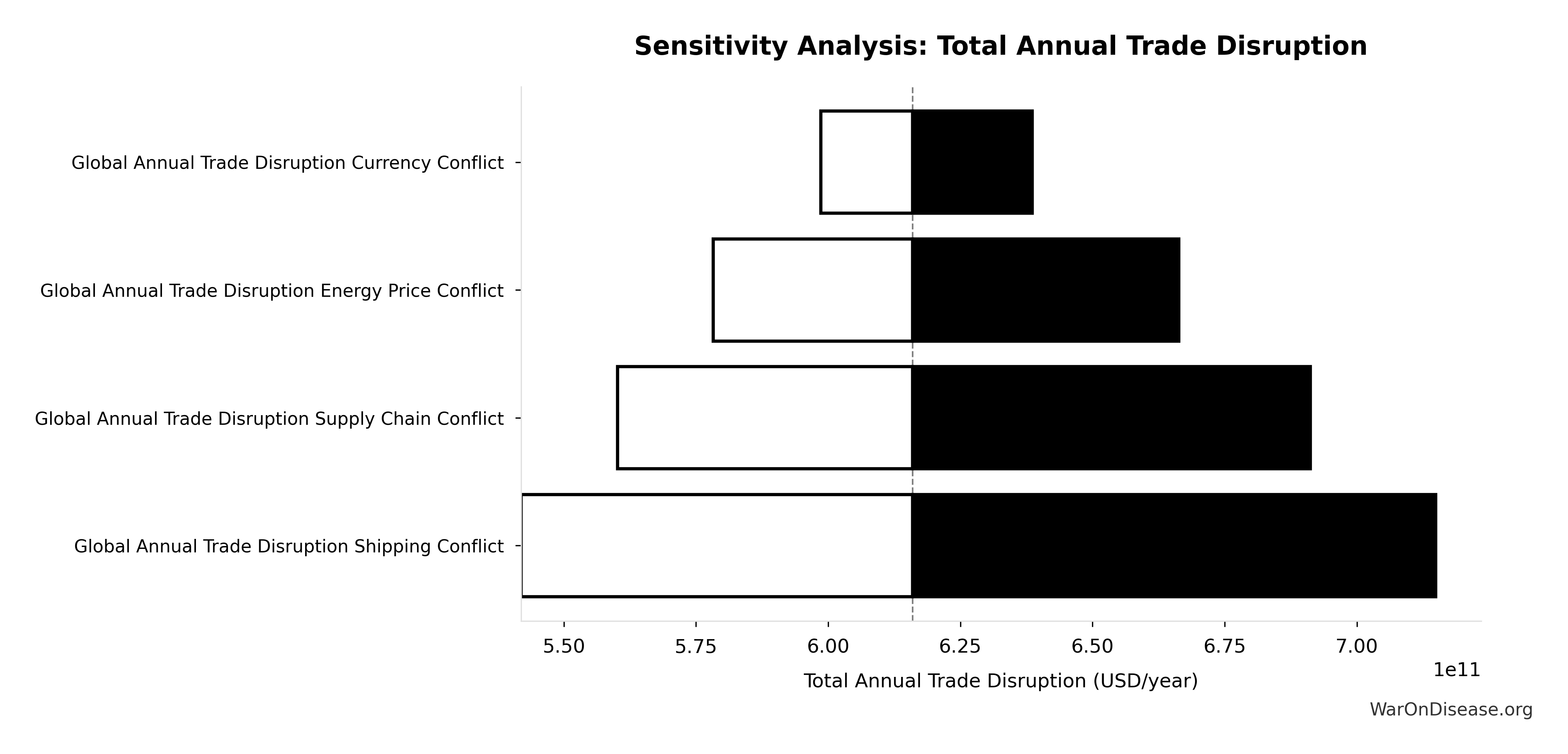
Simulation Results Summary: dFDA Trial Cost Reduction Percentage
| Statistic | Value |
|---|---|
| Baseline (deterministic) | 97.7% |
| Mean (expected value) | 98% |
| Median (50th percentile) | 97.9% |
| Standard Deviation | 0.401% |
| 90% Range (5th-95th percentile) | [97.5%, 98.9%] |
The histogram shows the distribution of dFDA Trial Cost Reduction Percentage across 10,000 Monte Carlo simulations. The CDF (right) shows the probability of the outcome exceeding any given value, which is useful for risk assessment.
Exceedance Probability
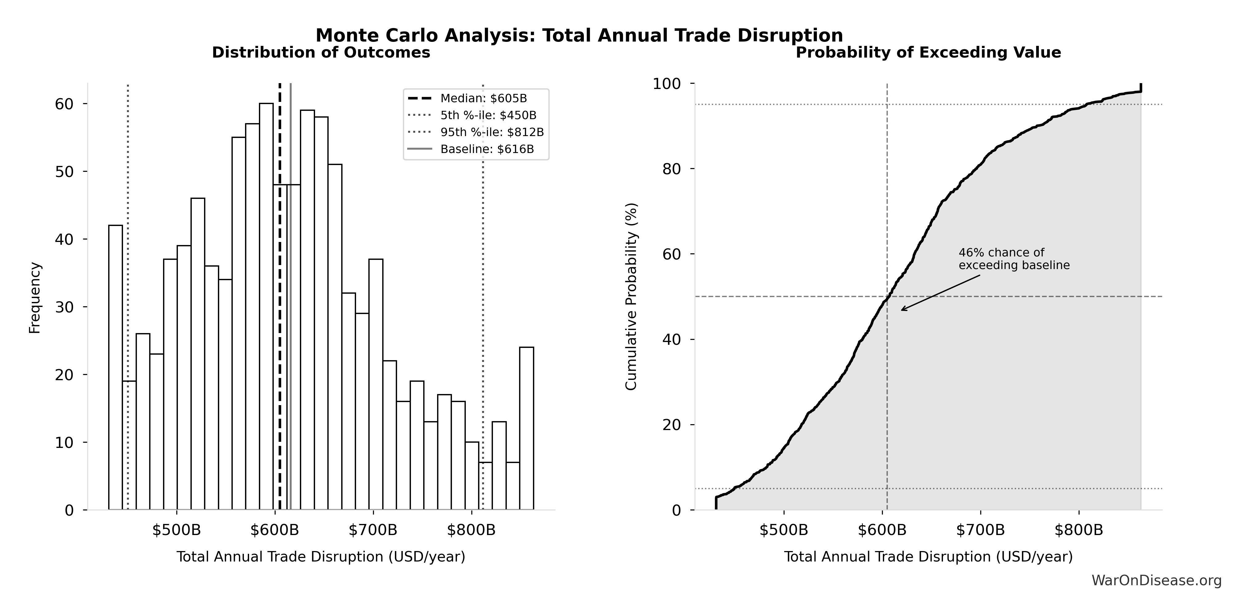
This exceedance probability chart shows the likelihood that dFDA Trial Cost Reduction Percentage will exceed any given threshold. Higher curves indicate more favorable outcomes with greater certainty.
dFDA Annual Trial Subsidies: $21.8B
Note📊 Details
Annual clinical trial patient subsidies from dFDA funding (total funding minus operational costs)
Inputs:
- dFDA Annual Trial Funding: $21.8B
- Total Annual Decentralized Framework for Drug Assessment Operational Costs 🔢: $40M
\[ \begin{gathered} Subsidies_{dFDA,ann} \\ = Funding_{dFDA,ann} - OPEX_{dFDA} \\ = \$21.8B - \$40M \\ = \$21.8B \end{gathered} \] where: \[ \begin{gathered} OPEX_{dFDA} \\ = Cost_{platform} + Cost_{staff} + Cost_{infra} \\ + Cost_{regulatory} + Cost_{community} \\ = \$15M + \$10M + \$8M + \$5M + \$2M \\ = \$40M \end{gathered} \] ✓ High confidence
Sensitivity Analysis
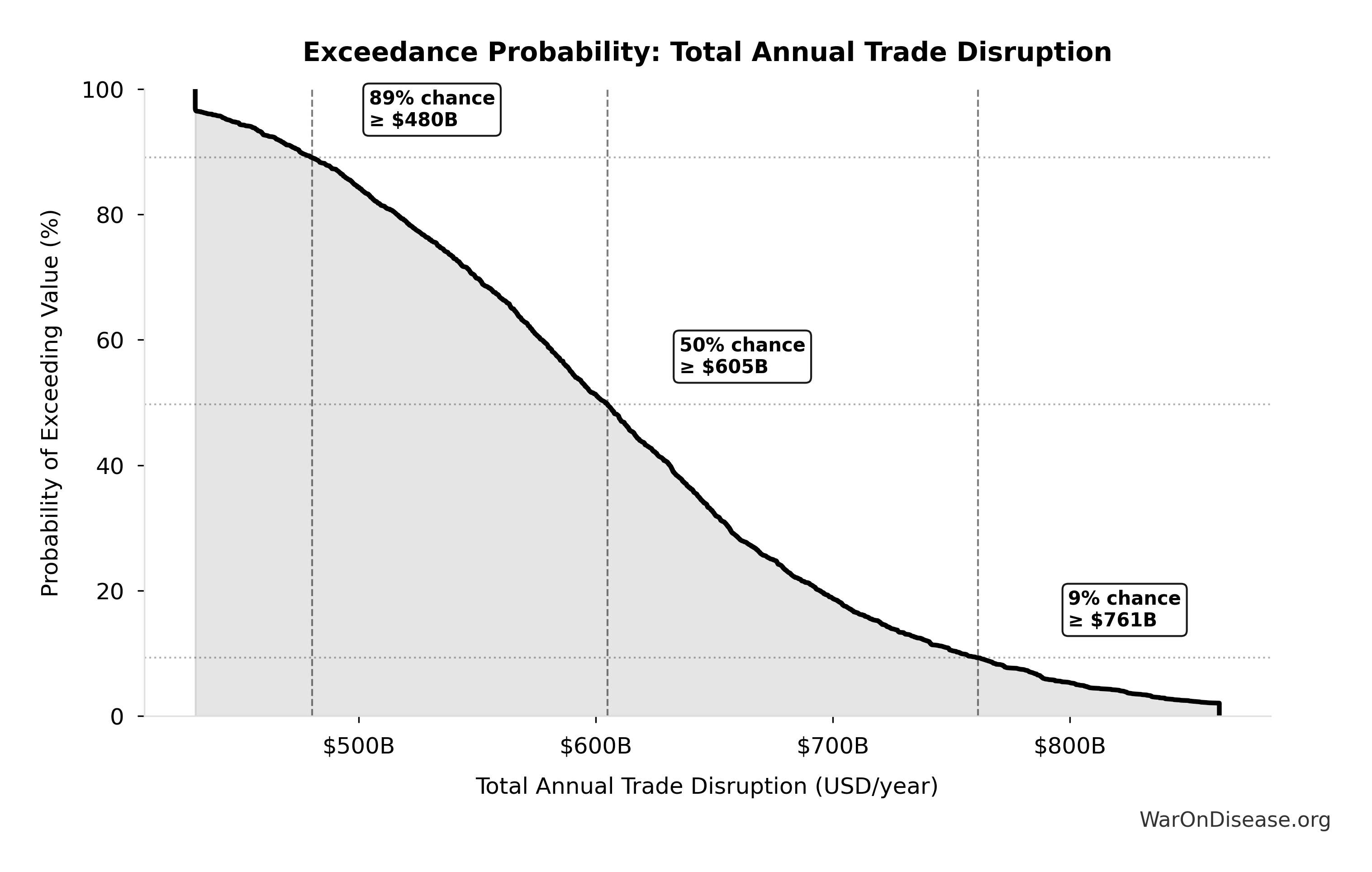
Sensitivity Indices for dFDA Annual Trial Subsidies
Regression-based sensitivity showing which inputs explain the most variance in the output.
| Input Parameter | Sensitivity Coefficient | Interpretation |
|---|---|---|
| Total Annual Decentralized Framework for Drug Assessment Operational Costs (USD/year) | -1.0000 | Strong driver |
Interpretation: Standardized coefficients show the change in output (in SD units) per 1 SD change in input. Values near ±1 indicate strong influence; values exceeding ±1 may occur with correlated inputs.
Monte Carlo Distribution
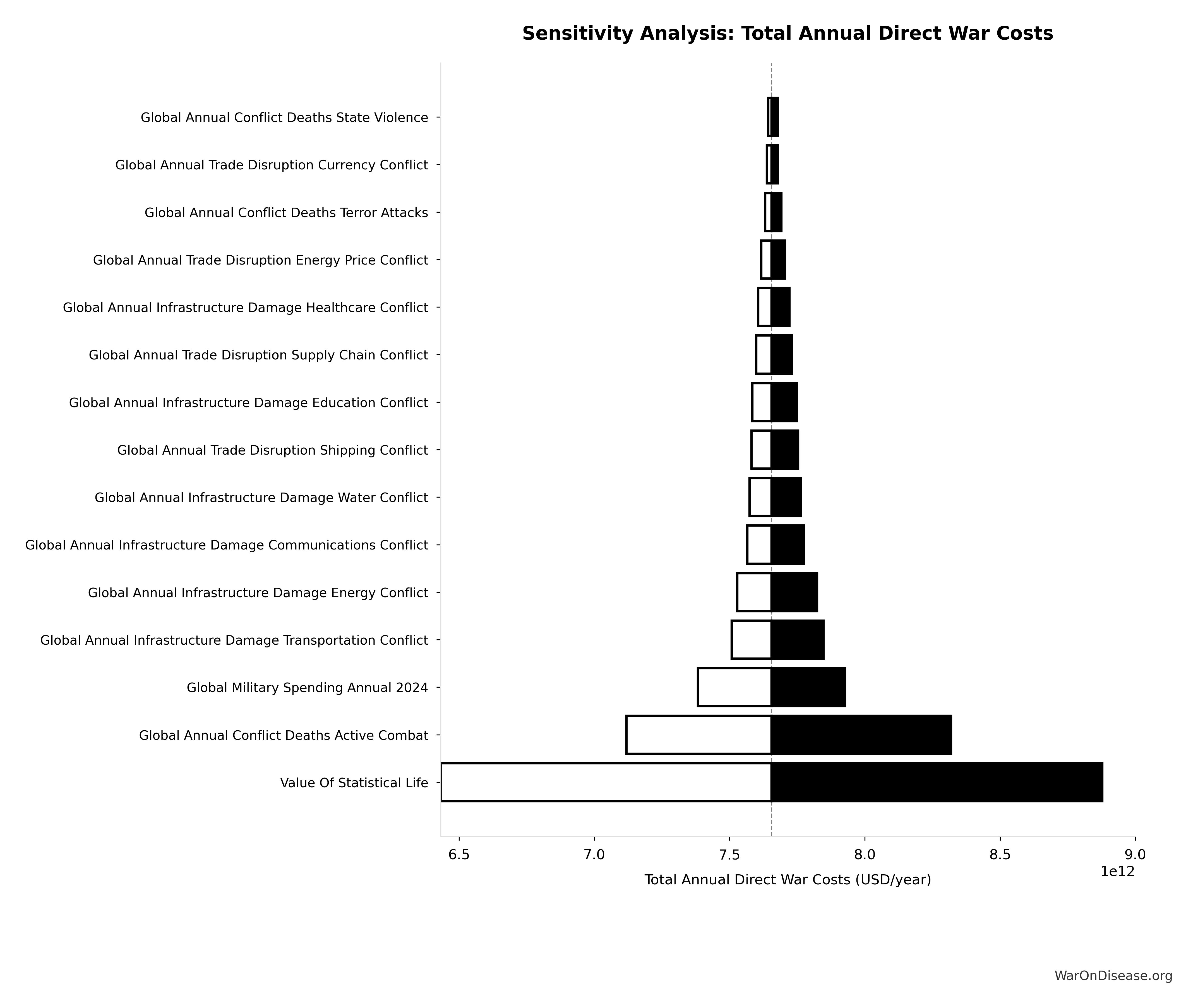
Simulation Results Summary: dFDA Annual Trial Subsidies
| Statistic | Value |
|---|---|
| Baseline (deterministic) | $21.8B |
| Mean (expected value) | $21.8B |
| Median (50th percentile) | $21.8B |
| Standard Deviation | $8.21M |
| 90% Range (5th-95th percentile) | [$21.7B, $21.8B] |
The histogram shows the distribution of dFDA Annual Trial Subsidies across 10,000 Monte Carlo simulations. The CDF (right) shows the probability of the outcome exceeding any given value, which is useful for risk assessment.
Exceedance Probability
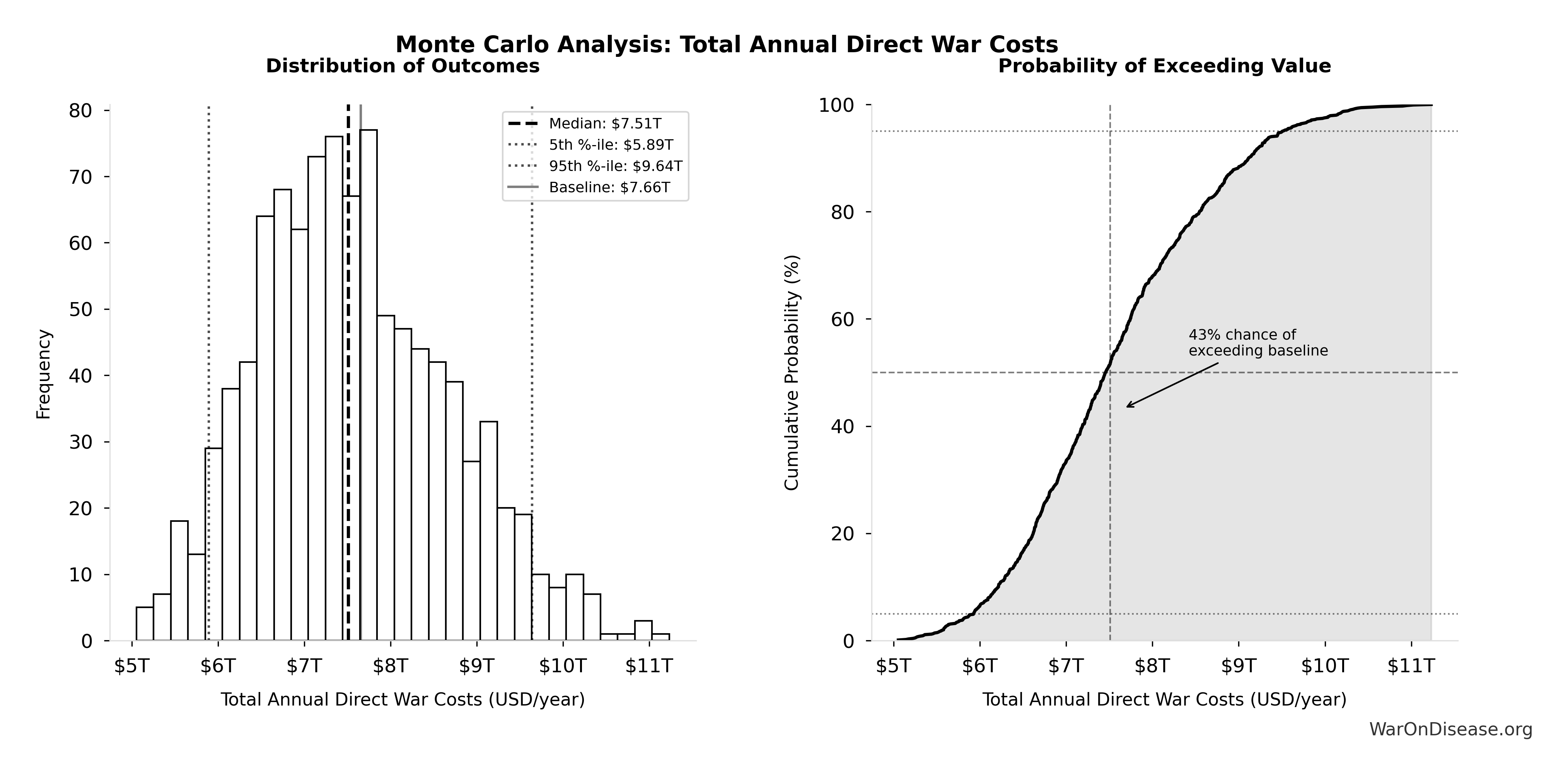
This exceedance probability chart shows the likelihood that dFDA Annual Trial Subsidies will exceed any given threshold. Higher curves indicate more favorable outcomes with greater certainty.
dFDA Valley of Death Rescue Multiplier: 1.4x
Note📊 Details
Factor increase in drugs entering development when dFDA eliminates Phase 2/3 cost barrier. Valley-of-death attrition (40%) becomes new drugs, so 1 + 0.40 = 1.4× more drugs.
Inputs:
- Valley of Death Attrition Rate 📊: 40% (95% CI: 25% - 55%)
\[ k_{rescue} = Attrition_{valley} + 1 = 40\% + 1 = 1.4 \]
~ Medium confidence
Sensitivity Analysis
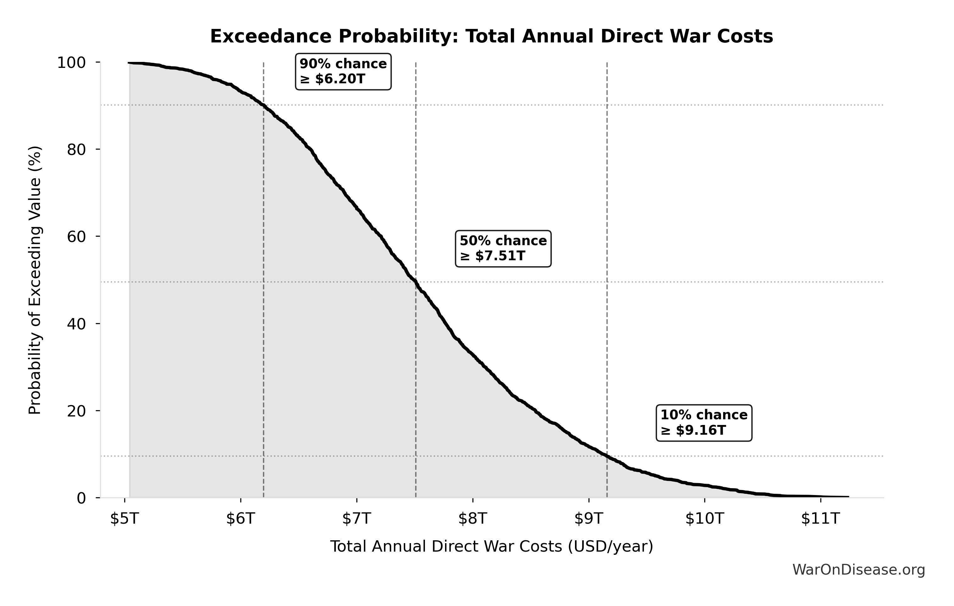
Monte Carlo Distribution
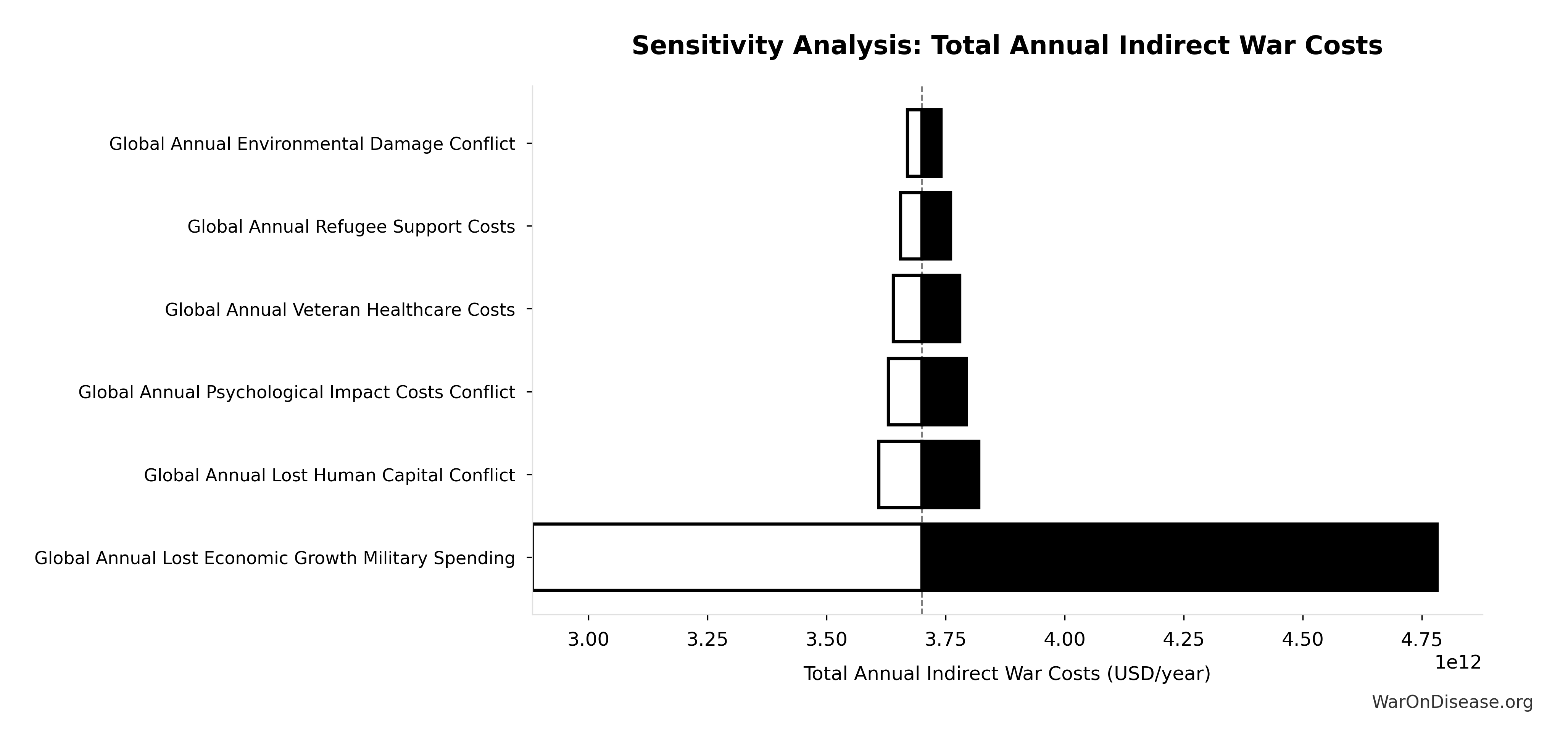
Simulation Results Summary: dFDA Valley of Death Rescue Multiplier
| Statistic | Value |
|---|---|
| Baseline (deterministic) | 1.4x |
| Mean (expected value) | 1.4x |
| Median (50th percentile) | 1.4x |
| Standard Deviation | 2.22e-16x |
| 90% Range (5th-95th percentile) | [1.4x, 1.4x] |
The histogram shows the distribution of dFDA Valley of Death Rescue Multiplier across 10,000 Monte Carlo simulations. The CDF (right) shows the probability of the outcome exceeding any given value, which is useful for risk assessment.
Exceedance Probability
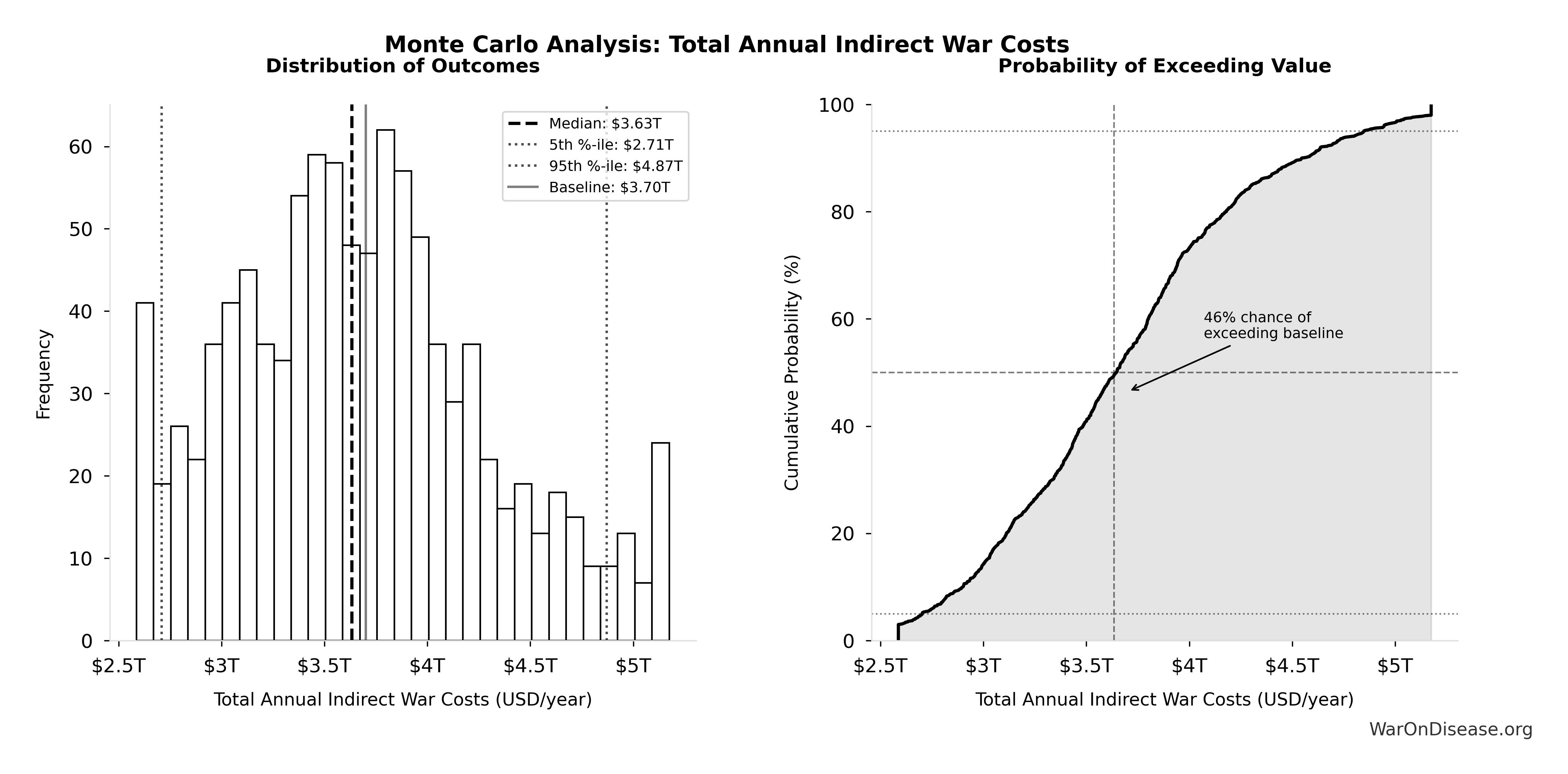
This exceedance probability chart shows the likelihood that dFDA Valley of Death Rescue Multiplier will exceed any given threshold. Higher curves indicate more favorable outcomes with greater certainty.
Patients Fundable Annually: 23.4 million patients/year
Note📊 Details
Number of patients fundable annually at dFDA pragmatic trial cost. Based on empirical pragmatic trial costs (RECOVERY to PCORnet range).
Inputs:
- Annual Clinical Trial Patient Subsidies 🔢: $21.7B
- dFDA Pragmatic Trial Cost per Patient 📊: $929 (95% CI: $97 - $3K)
\[ \begin{gathered} N_{fundable,ann} \\ = \frac{Subsidies_{trial,ann}}{Cost_{pragmatic,pt}} \\ = \frac{\$21.7B}{\$929} \\ = 23.4M \end{gathered} \] where: \[ \begin{gathered} Subsidies_{trial,ann} \\ = Treasury_{RD,ann} - OPEX_{dFDA} \\ = \$21.8B - \$40M \\ = \$21.7B \end{gathered} \] where: \[ \begin{gathered} OPEX_{dFDA} \\ = Cost_{platform} + Cost_{staff} + Cost_{infra} \\ + Cost_{regulatory} + Cost_{community} \\ = \$15M + \$10M + \$8M + \$5M + \$2M \\ = \$40M \end{gathered} \] where: \[ \begin{gathered} Treasury_{RD,ann} \\ = Funding_{treaty} - Payout_{bond,ann} - Funding_{political,ann} \\ = \$27.2B - \$2.72B - \$2.72B \\ = \$21.8B \end{gathered} \] where: \[ \begin{gathered} Funding_{treaty} \\ = Spending_{mil} \times Reduce_{treaty} \\ = \$2.72T \times 1\% \\ = \$27.2B \end{gathered} \] where: \[ \begin{gathered} Payout_{bond,ann} \\ = Funding_{treaty} \times Pct_{bond} \\ = \$27.2B \times 10\% \\ = \$2.72B \end{gathered} \] where: \[ \begin{gathered} Funding_{political,ann} \\ = Funding_{treaty} \times Pct_{political} \\ = \$27.2B \times 10\% \\ = \$2.72B \end{gathered} \] ✓ High confidence
Sensitivity Analysis
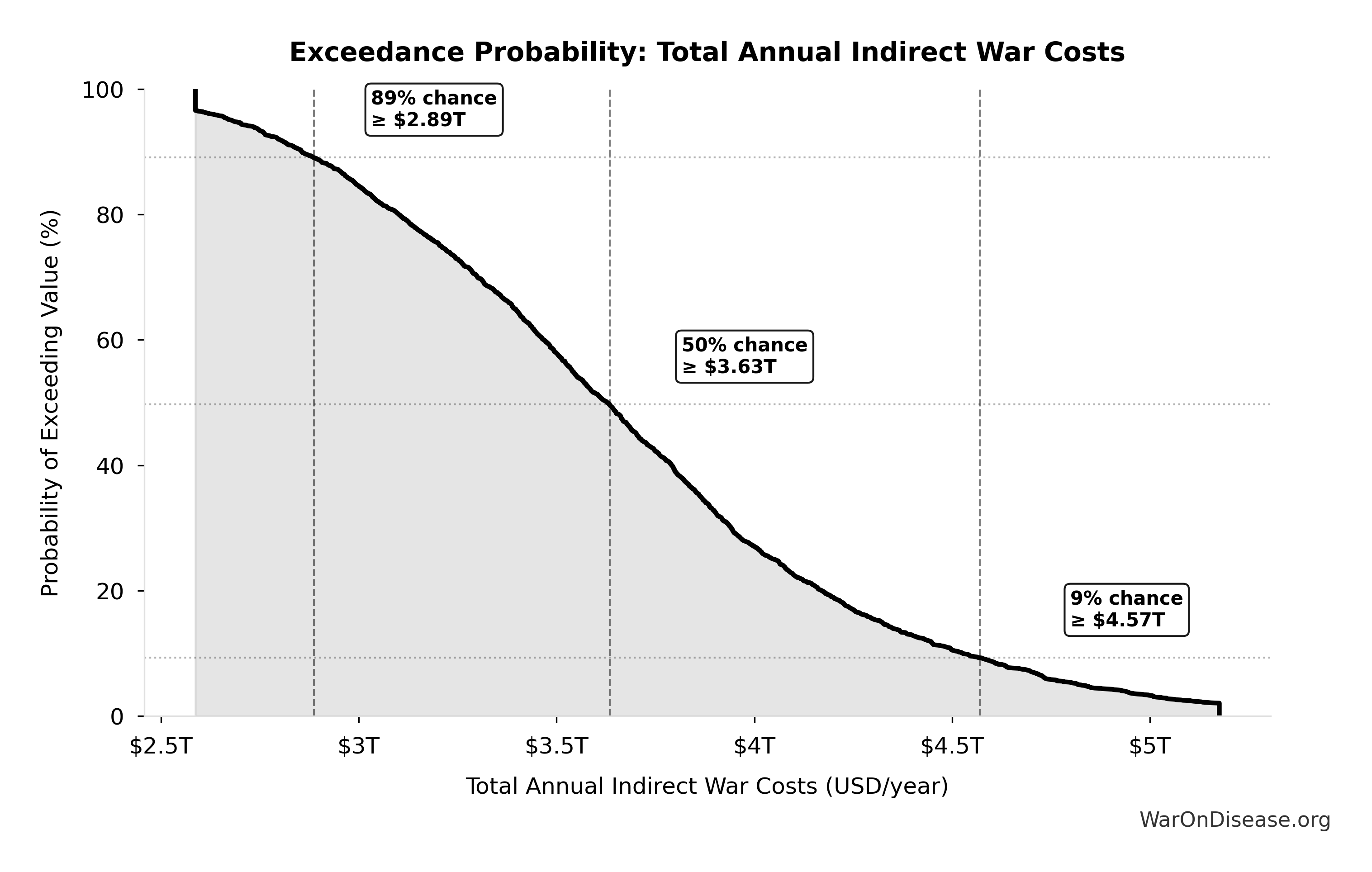
Sensitivity Indices for Patients Fundable Annually
Regression-based sensitivity showing which inputs explain the most variance in the output.
| Input Parameter | Sensitivity Coefficient | Interpretation |
|---|---|---|
| Annual Clinical Trial Patient Subsidies (USD/year) | 2.3351 | Strong driver |
| dFDA Pragmatic Trial Cost per Patient (USD/patient) | 1.5755 | Strong driver |
Interpretation: Standardized coefficients show the change in output (in SD units) per 1 SD change in input. Values near ±1 indicate strong influence; values exceeding ±1 may occur with correlated inputs.
Monte Carlo Distribution
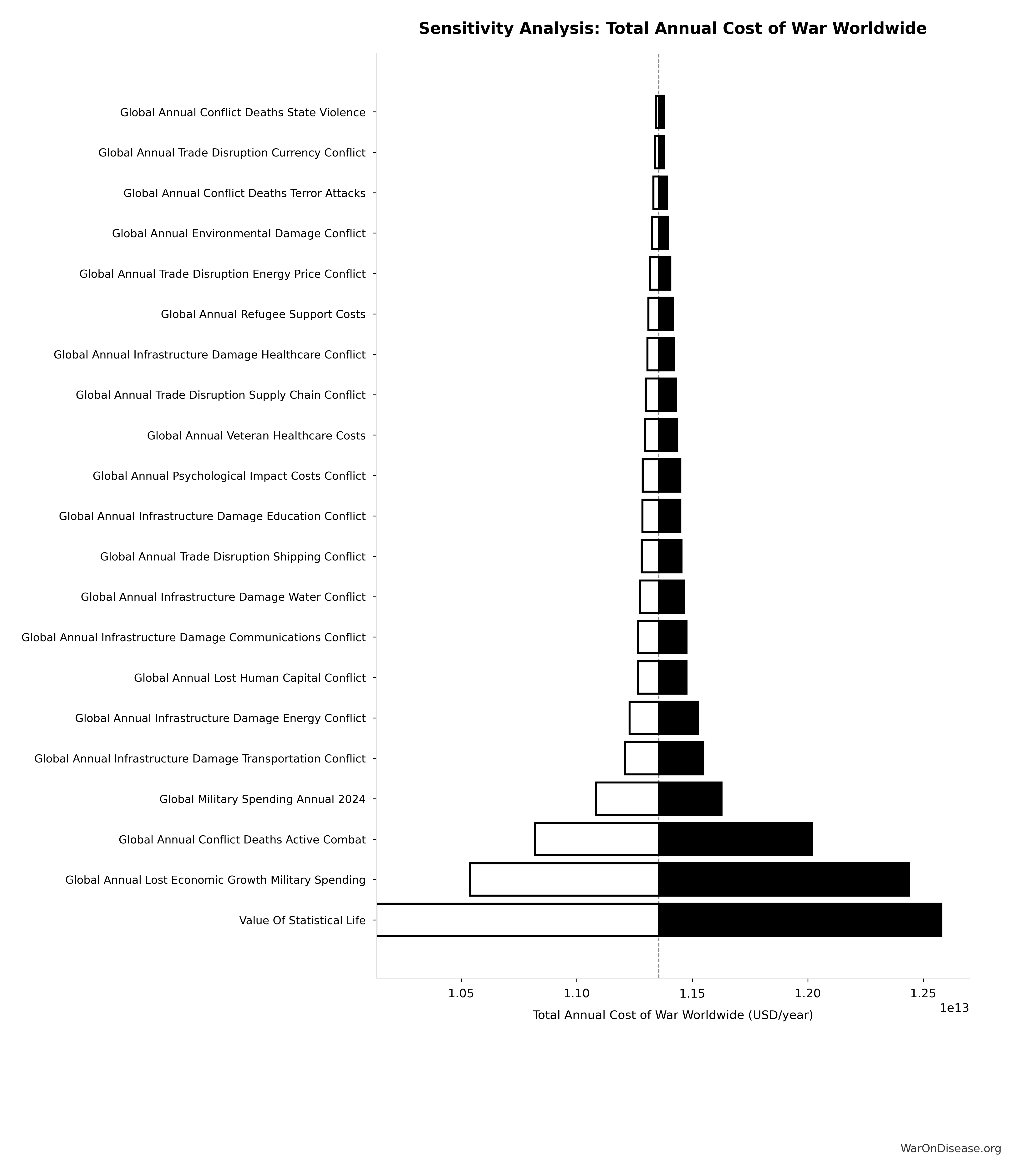
Simulation Results Summary: Patients Fundable Annually
| Statistic | Value |
|---|---|
| Baseline (deterministic) | 23.4 million |
| Mean (expected value) | 38.6 million |
| Median (50th percentile) | 30.2 million |
| Standard Deviation | 30.2 million |
| 90% Range (5th-95th percentile) | [9.44 million, 96.8 million] |
The histogram shows the distribution of Patients Fundable Annually across 10,000 Monte Carlo simulations. The CDF (right) shows the probability of the outcome exceeding any given value, which is useful for risk assessment.
Exceedance Probability
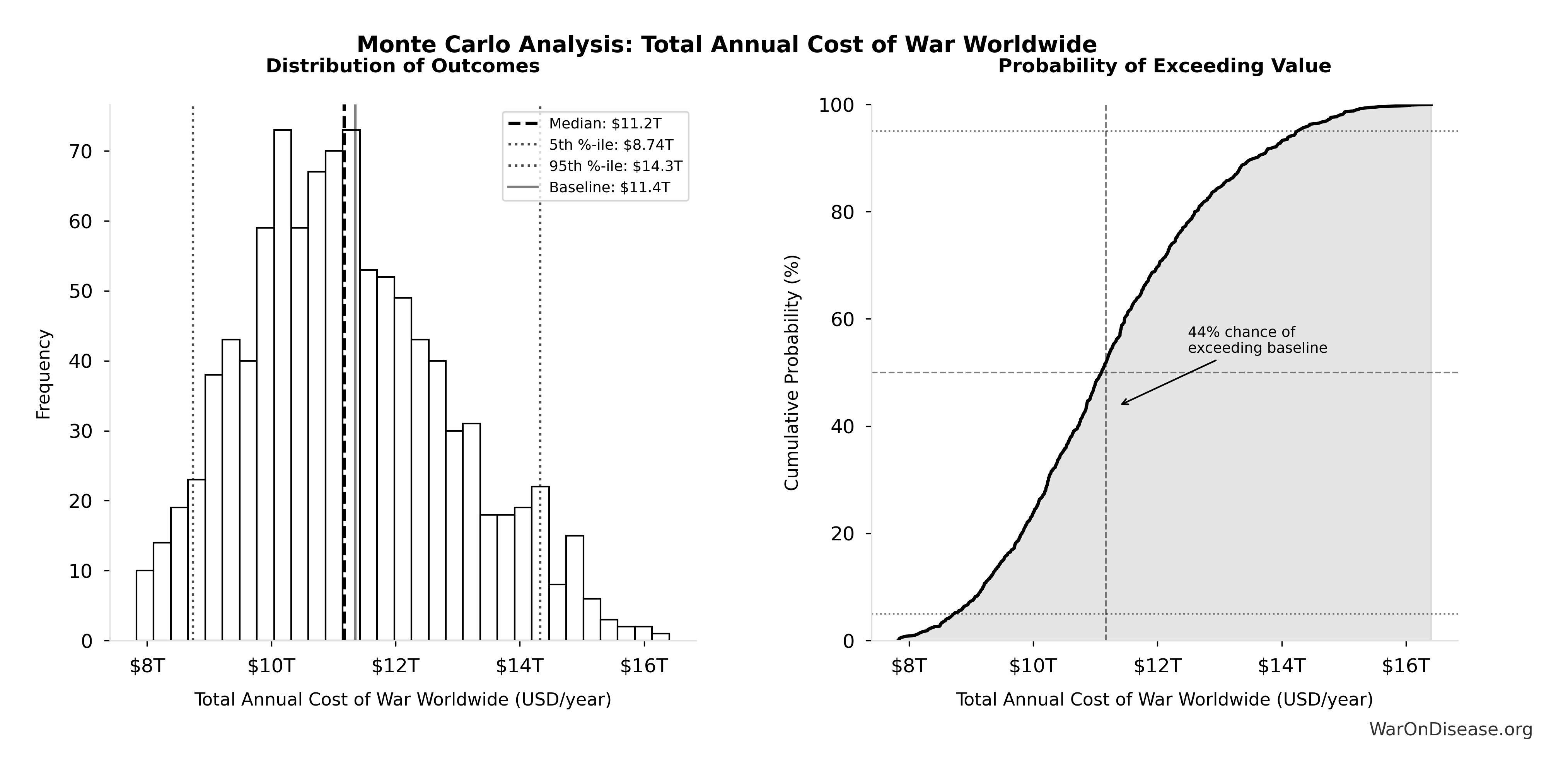
This exceedance probability chart shows the likelihood that Patients Fundable Annually will exceed any given threshold. Higher curves indicate more favorable outcomes with greater certainty.
Medical Research Percentage of Treaty Funding: 80%
Note📊 Details
Percentage of treaty funding allocated to medical research (after bond payouts and IAB incentives)
Inputs:
- Annual Funding for Pragmatic Clinical Trials 🔢: $21.8B
- Annual Funding from 1% of Global Military Spending Redirected to DIH 🔢: $27.2B
\[ \begin{gathered} Pct_{treasury,RD} \\ = \frac{Treasury_{RD,ann}}{Funding_{treaty}} \\ = \frac{\$21.8B}{\$27.2B} \\ = 80\% \end{gathered} \] where: \[ \begin{gathered} Treasury_{RD,ann} \\ = Funding_{treaty} - Payout_{bond,ann} - Funding_{political,ann} \\ = \$27.2B - \$2.72B - \$2.72B \\ = \$21.8B \end{gathered} \] where: \[ \begin{gathered} Funding_{treaty} \\ = Spending_{mil} \times Reduce_{treaty} \\ = \$2.72T \times 1\% \\ = \$27.2B \end{gathered} \] where: \[ \begin{gathered} Payout_{bond,ann} \\ = Funding_{treaty} \times Pct_{bond} \\ = \$27.2B \times 10\% \\ = \$2.72B \end{gathered} \] where: \[ \begin{gathered} Funding_{political,ann} \\ = Funding_{treaty} \times Pct_{political} \\ = \$27.2B \times 10\% \\ = \$2.72B \end{gathered} \] ✓ High confidence
Monte Carlo Distribution
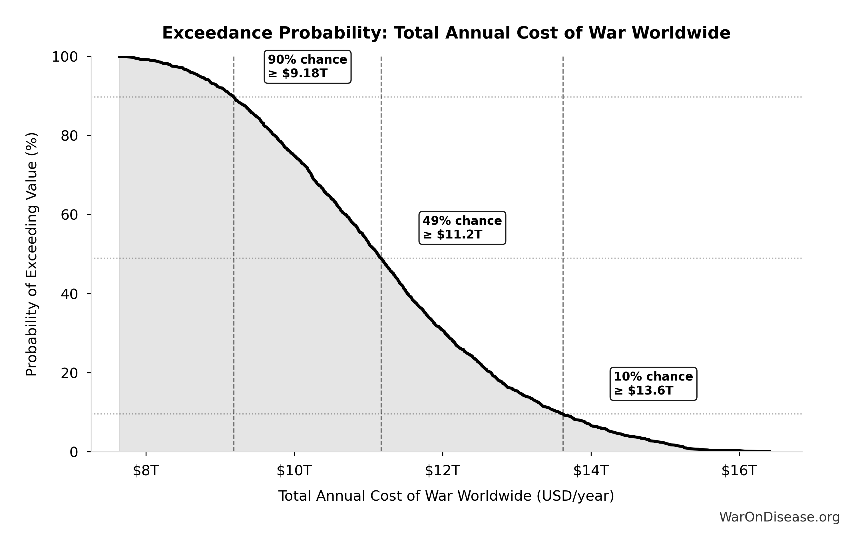
Simulation Results Summary: Medical Research Percentage of Treaty Funding
| Statistic | Value |
|---|---|
| Baseline (deterministic) | 80% |
| Mean (expected value) | 80% |
| Median (50th percentile) | 80% |
| Standard Deviation | 1.11e-14% |
| 90% Range (5th-95th percentile) | [80%, 80%] |
The histogram shows the distribution of Medical Research Percentage of Treaty Funding across 10,000 Monte Carlo simulations. The CDF (right) shows the probability of the outcome exceeding any given value, which is useful for risk assessment.
Exceedance Probability
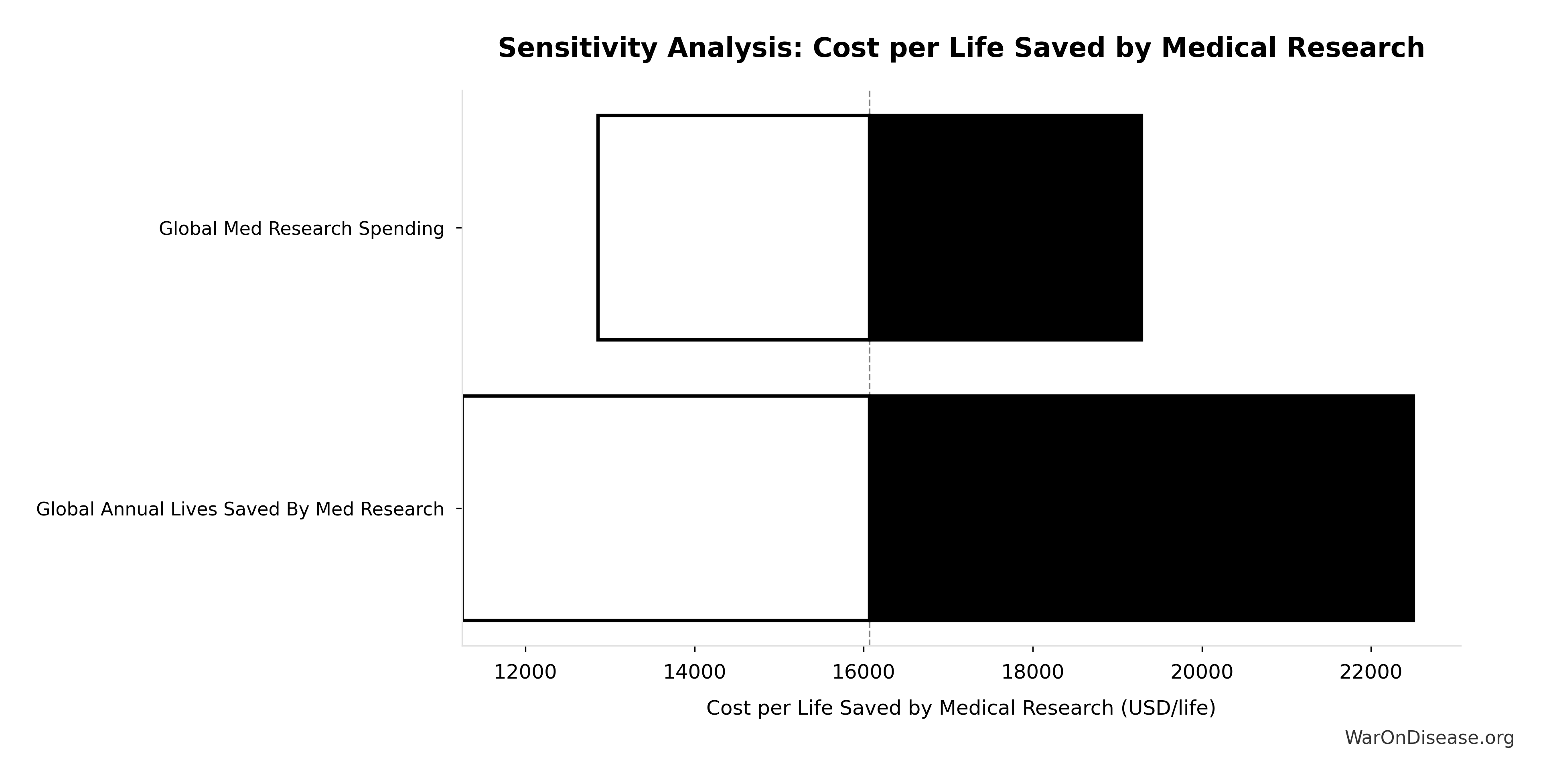
This exceedance probability chart shows the likelihood that Medical Research Percentage of Treaty Funding will exceed any given threshold. Higher curves indicate more favorable outcomes with greater certainty.
Annual Funding for Pragmatic Clinical Trials: $21.8B
Note📊 Details
Annual funding for pragmatic clinical trials (treaty funding minus VICTORY Incentive Alignment Bond payouts and IAB political incentive mechanism)
Inputs:
- Annual Funding from 1% of Global Military Spending Redirected to DIH 🔢: $27.2B
- Annual VICTORY Incentive Alignment Bond Payout 🔢: $2.72B
- Annual IAB Political Incentive Funding 🔢: $2.72B
\[ \begin{gathered} Treasury_{RD,ann} \\ = Funding_{treaty} - Payout_{bond,ann} - Funding_{political,ann} \\ = \$27.2B - \$2.72B - \$2.72B \\ = \$21.8B \end{gathered} \] where: \[ \begin{gathered} Funding_{treaty} \\ = Spending_{mil} \times Reduce_{treaty} \\ = \$2.72T \times 1\% \\ = \$27.2B \end{gathered} \] where: \[ \begin{gathered} Payout_{bond,ann} \\ = Funding_{treaty} \times Pct_{bond} \\ = \$27.2B \times 10\% \\ = \$2.72B \end{gathered} \] where: \[ \begin{gathered} Funding_{political,ann} \\ = Funding_{treaty} \times Pct_{political} \\ = \$27.2B \times 10\% \\ = \$2.72B \end{gathered} \] ✓ High confidence
Annual Clinical Trial Patient Subsidies: $21.7B
Note📊 Details
Annual clinical trial patient subsidies (all medical research funds after Decentralized Framework for Drug Assessment operations)
Inputs:
- Total Annual Decentralized Framework for Drug Assessment Operational Costs 🔢: $40M
- Annual Funding for Pragmatic Clinical Trials 🔢: $21.8B
\[ \begin{gathered} Subsidies_{trial,ann} \\ = Treasury_{RD,ann} - OPEX_{dFDA} \\ = \$21.8B - \$40M \\ = \$21.7B \end{gathered} \] where: \[ \begin{gathered} OPEX_{dFDA} \\ = Cost_{platform} + Cost_{staff} + Cost_{infra} \\ + Cost_{regulatory} + Cost_{community} \\ = \$15M + \$10M + \$8M + \$5M + \$2M \\ = \$40M \end{gathered} \] where: \[ \begin{gathered} Treasury_{RD,ann} \\ = Funding_{treaty} - Payout_{bond,ann} - Funding_{political,ann} \\ = \$27.2B - \$2.72B - \$2.72B \\ = \$21.8B \end{gathered} \] where: \[ \begin{gathered} Funding_{treaty} \\ = Spending_{mil} \times Reduce_{treaty} \\ = \$2.72T \times 1\% \\ = \$27.2B \end{gathered} \] where: \[ \begin{gathered} Payout_{bond,ann} \\ = Funding_{treaty} \times Pct_{bond} \\ = \$27.2B \times 10\% \\ = \$2.72B \end{gathered} \] where: \[ \begin{gathered} Funding_{political,ann} \\ = Funding_{treaty} \times Pct_{political} \\ = \$27.2B \times 10\% \\ = \$2.72B \end{gathered} \] ✓ High confidence
Sensitivity Analysis
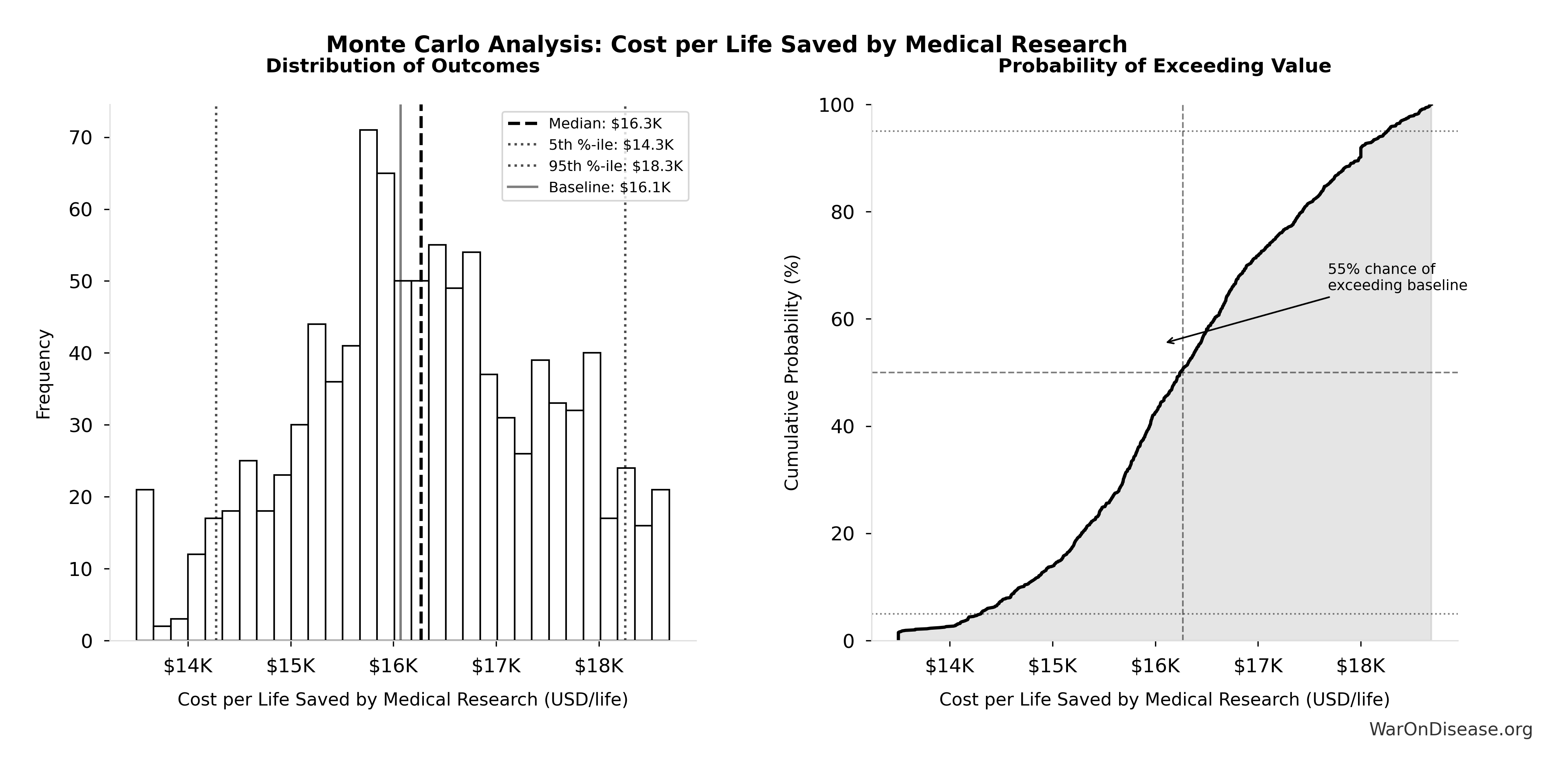
Sensitivity Indices for Annual Clinical Trial Patient Subsidies
Regression-based sensitivity showing which inputs explain the most variance in the output.
| Input Parameter | Sensitivity Coefficient | Interpretation |
|---|---|---|
| Total Annual Decentralized Framework for Drug Assessment Operational Costs (USD/year) | -1.0000 | Strong driver |
Interpretation: Standardized coefficients show the change in output (in SD units) per 1 SD change in input. Values near ±1 indicate strong influence; values exceeding ±1 may occur with correlated inputs.
Monte Carlo Distribution
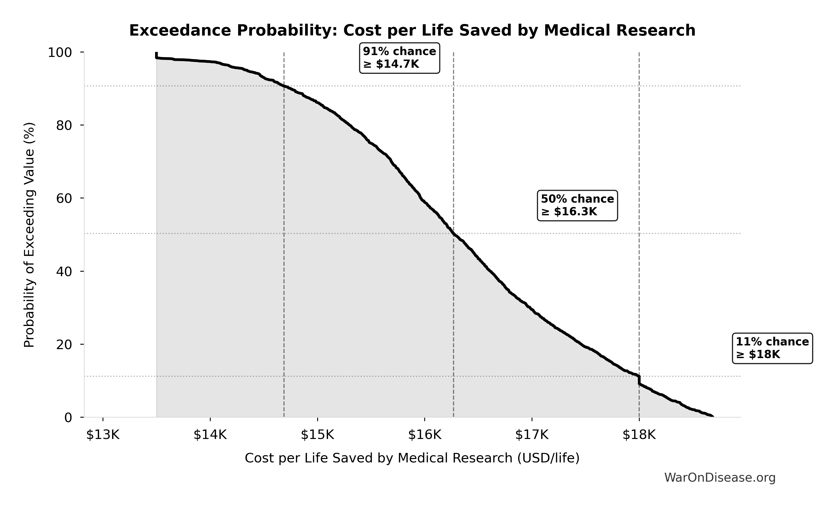
Simulation Results Summary: Annual Clinical Trial Patient Subsidies
| Statistic | Value |
|---|---|
| Baseline (deterministic) | $21.7B |
| Mean (expected value) | $21.7B |
| Median (50th percentile) | $21.7B |
| Standard Deviation | $8.21M |
| 90% Range (5th-95th percentile) | [$21.7B, $21.7B] |
The histogram shows the distribution of Annual Clinical Trial Patient Subsidies across 10,000 Monte Carlo simulations. The CDF (right) shows the probability of the outcome exceeding any given value, which is useful for risk assessment.
Exceedance Probability
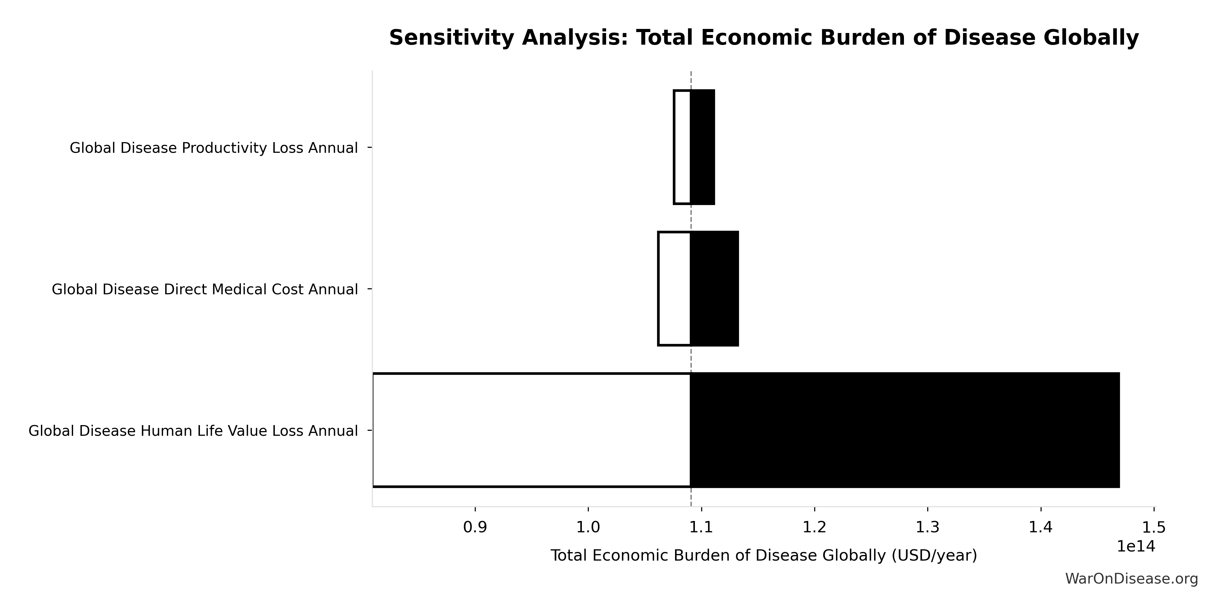
This exceedance probability chart shows the likelihood that Annual Clinical Trial Patient Subsidies will exceed any given threshold. Higher curves indicate more favorable outcomes with greater certainty.
Patient Trial Subsidies Percentage of Treaty Funding: 79.9%
Note📊 Details
Percentage of treaty funding going directly to patient trial subsidies
Inputs:
- Annual Clinical Trial Patient Subsidies 🔢: $21.7B
- Annual Funding from 1% of Global Military Spending Redirected to DIH 🔢: $27.2B
\[ \begin{gathered} Pct_{subsidies} \\ = \frac{Subsidies_{trial,ann}}{Funding_{treaty}} \\ = \frac{\$21.7B}{\$27.2B} \\ = 79.9\% \end{gathered} \] where: \[ \begin{gathered} Subsidies_{trial,ann} \\ = Treasury_{RD,ann} - OPEX_{dFDA} \\ = \$21.8B - \$40M \\ = \$21.7B \end{gathered} \] where: \[ \begin{gathered} OPEX_{dFDA} \\ = Cost_{platform} + Cost_{staff} + Cost_{infra} \\ + Cost_{regulatory} + Cost_{community} \\ = \$15M + \$10M + \$8M + \$5M + \$2M \\ = \$40M \end{gathered} \] where: \[ \begin{gathered} Treasury_{RD,ann} \\ = Funding_{treaty} - Payout_{bond,ann} - Funding_{political,ann} \\ = \$27.2B - \$2.72B - \$2.72B \\ = \$21.8B \end{gathered} \] where: \[ \begin{gathered} Funding_{treaty} \\ = Spending_{mil} \times Reduce_{treaty} \\ = \$2.72T \times 1\% \\ = \$27.2B \end{gathered} \] where: \[ \begin{gathered} Payout_{bond,ann} \\ = Funding_{treaty} \times Pct_{bond} \\ = \$27.2B \times 10\% \\ = \$2.72B \end{gathered} \] where: \[ \begin{gathered} Funding_{political,ann} \\ = Funding_{treaty} \times Pct_{political} \\ = \$27.2B \times 10\% \\ = \$2.72B \end{gathered} \] ✓ High confidence
Sensitivity Analysis
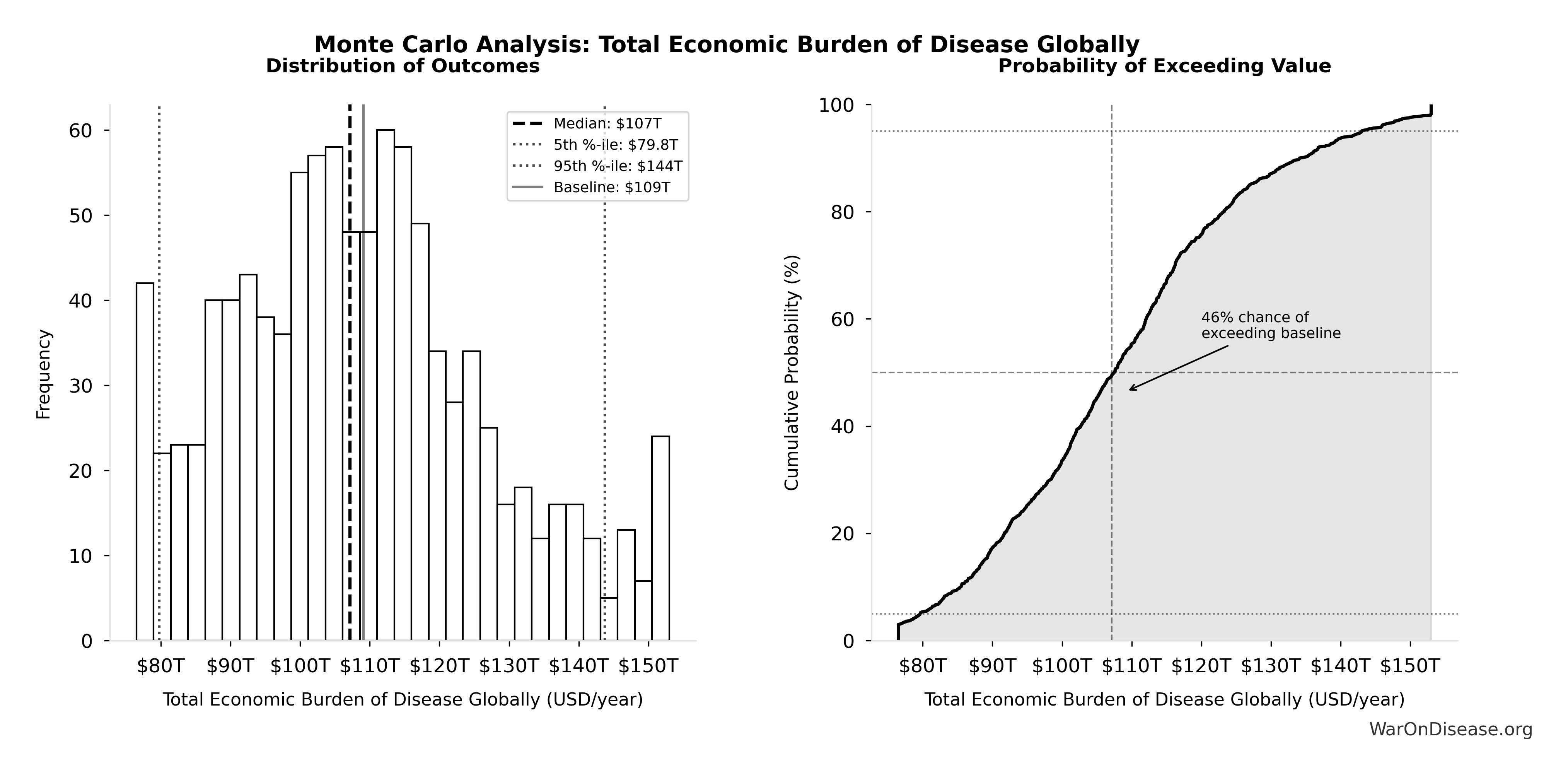
Sensitivity Indices for Patient Trial Subsidies Percentage of Treaty Funding
Regression-based sensitivity showing which inputs explain the most variance in the output.
| Input Parameter | Sensitivity Coefficient | Interpretation |
|---|---|---|
| Annual Clinical Trial Patient Subsidies (USD/year) | 1.0000 | Strong driver |
Interpretation: Standardized coefficients show the change in output (in SD units) per 1 SD change in input. Values near ±1 indicate strong influence; values exceeding ±1 may occur with correlated inputs.
Monte Carlo Distribution
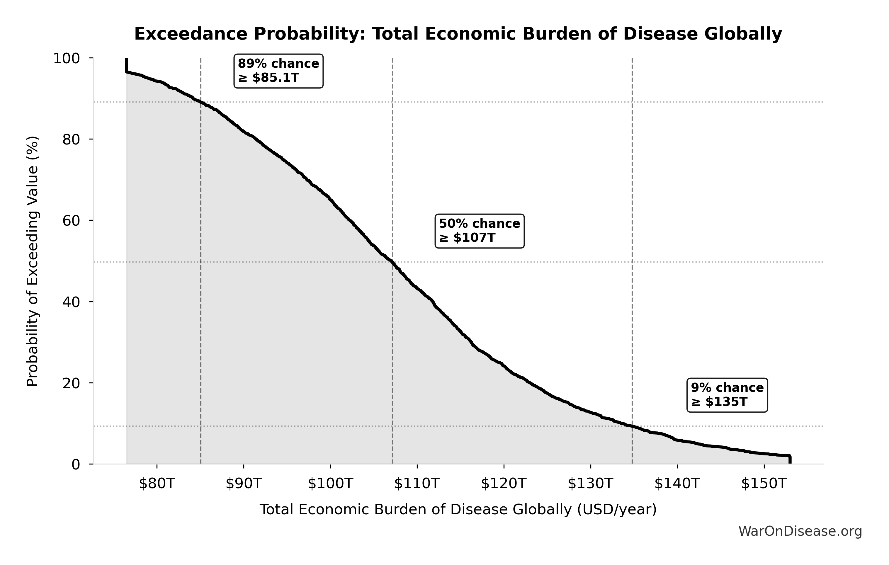
Simulation Results Summary: Patient Trial Subsidies Percentage of Treaty Funding
| Statistic | Value |
|---|---|
| Baseline (deterministic) | 79.9% |
| Mean (expected value) | 79.9% |
| Median (50th percentile) | 79.9% |
| Standard Deviation | 0.0302% |
| 90% Range (5th-95th percentile) | [79.8%, 79.9%] |
The histogram shows the distribution of Patient Trial Subsidies Percentage of Treaty Funding across 10,000 Monte Carlo simulations. The CDF (right) shows the probability of the outcome exceeding any given value, which is useful for risk assessment.
Exceedance Probability
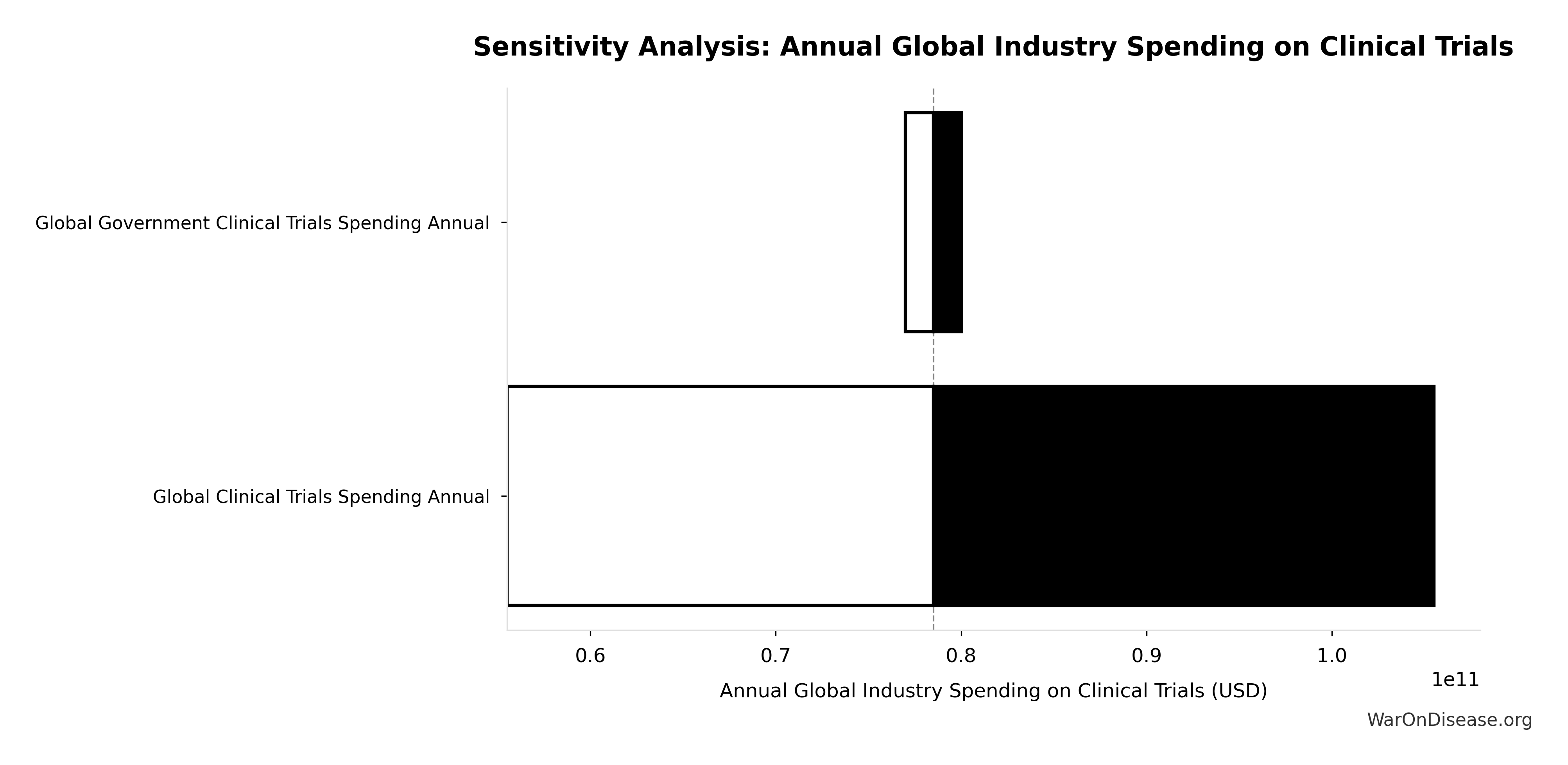
This exceedance probability chart shows the likelihood that Patient Trial Subsidies Percentage of Treaty Funding will exceed any given threshold. Higher curves indicate more favorable outcomes with greater certainty.
Diseases Without Effective Treatment: 6.65 thousand diseases
Note📊 Details
Number of diseases without effective treatment. 95% of 7,000 rare diseases lack FDA-approved treatment (per Orphanet 2024). This represents the therapeutic search space that remains unexplored.
Inputs:
- Total Number of Rare Diseases Globally 📊: 7 thousand diseases (95% CI: 6 thousand diseases - 10 thousand diseases)
\[ \begin{gathered} N_{untreated} \\ = N_{rare} \times 0.95 \\ = 7{,}000 \times 0.95 \\ = 6{,}650 \end{gathered} \]
Methodology:139
~ Medium confidence
Sensitivity Analysis
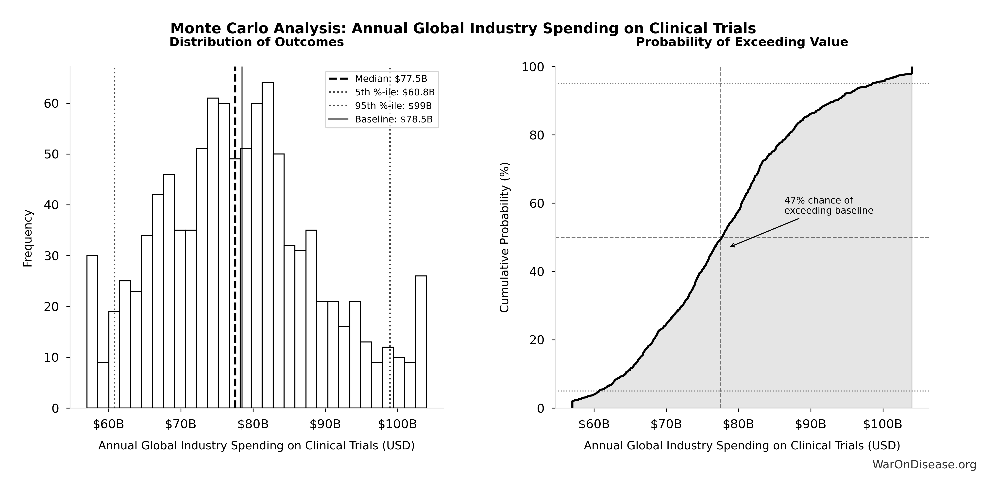
Sensitivity Indices for Diseases Without Effective Treatment
Regression-based sensitivity showing which inputs explain the most variance in the output.
| Input Parameter | Sensitivity Coefficient | Interpretation |
|---|---|---|
| Total Number of Rare Diseases Globally (diseases) | 1.0000 | Strong driver |
Interpretation: Standardized coefficients show the change in output (in SD units) per 1 SD change in input. Values near ±1 indicate strong influence; values exceeding ±1 may occur with correlated inputs.
Monte Carlo Distribution
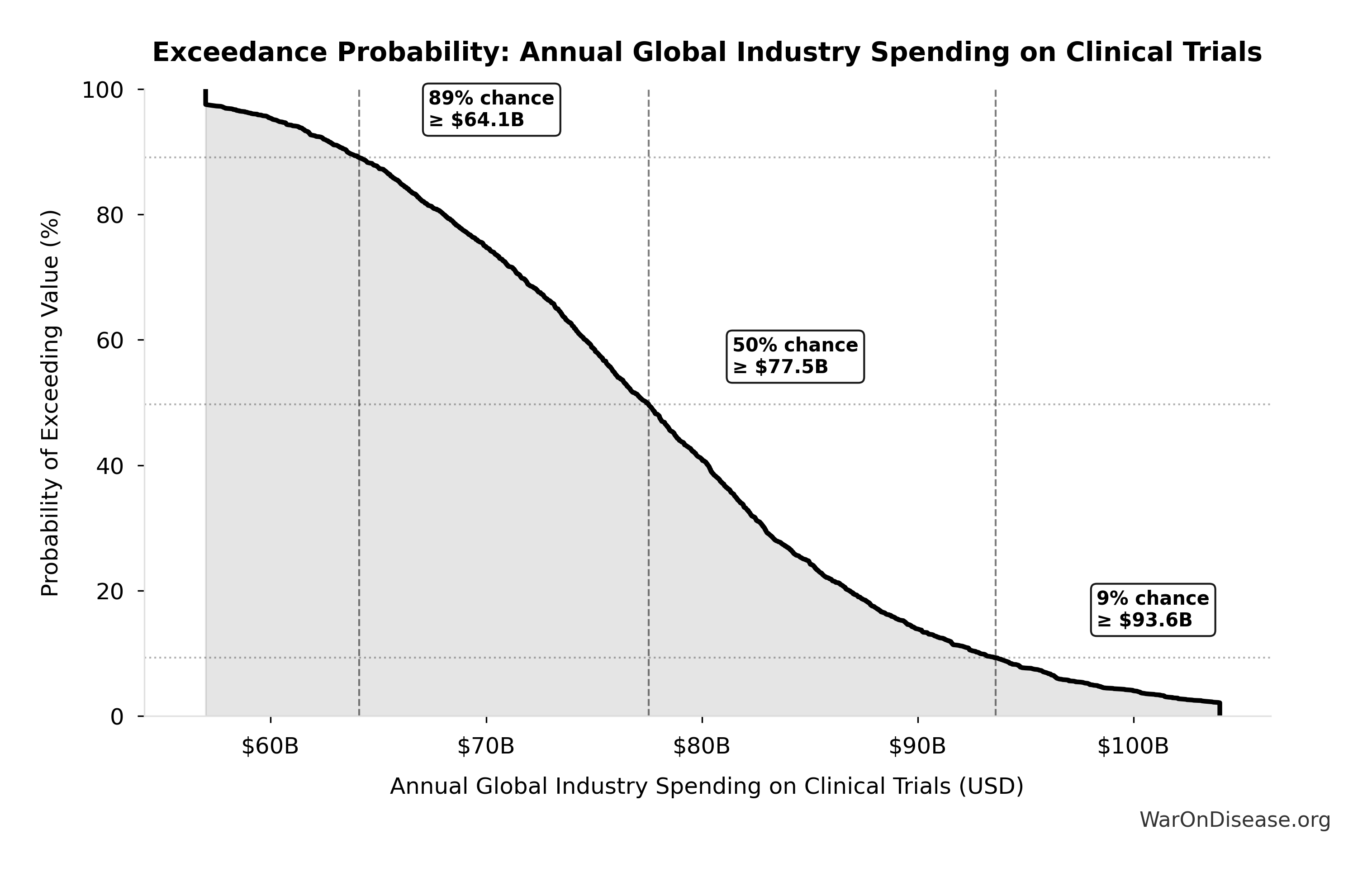
Simulation Results Summary: Diseases Without Effective Treatment
| Statistic | Value |
|---|---|
| Baseline (deterministic) | 6.65 thousand |
| Mean (expected value) | 6.73 thousand |
| Median (50th percentile) | 6.64 thousand |
| Standard Deviation | 835 |
| 90% Range (5th-95th percentile) | [5.7 thousand, 8.24 thousand] |
The histogram shows the distribution of Diseases Without Effective Treatment across 10,000 Monte Carlo simulations. The CDF (right) shows the probability of the outcome exceeding any given value, which is useful for risk assessment.
Exceedance Probability
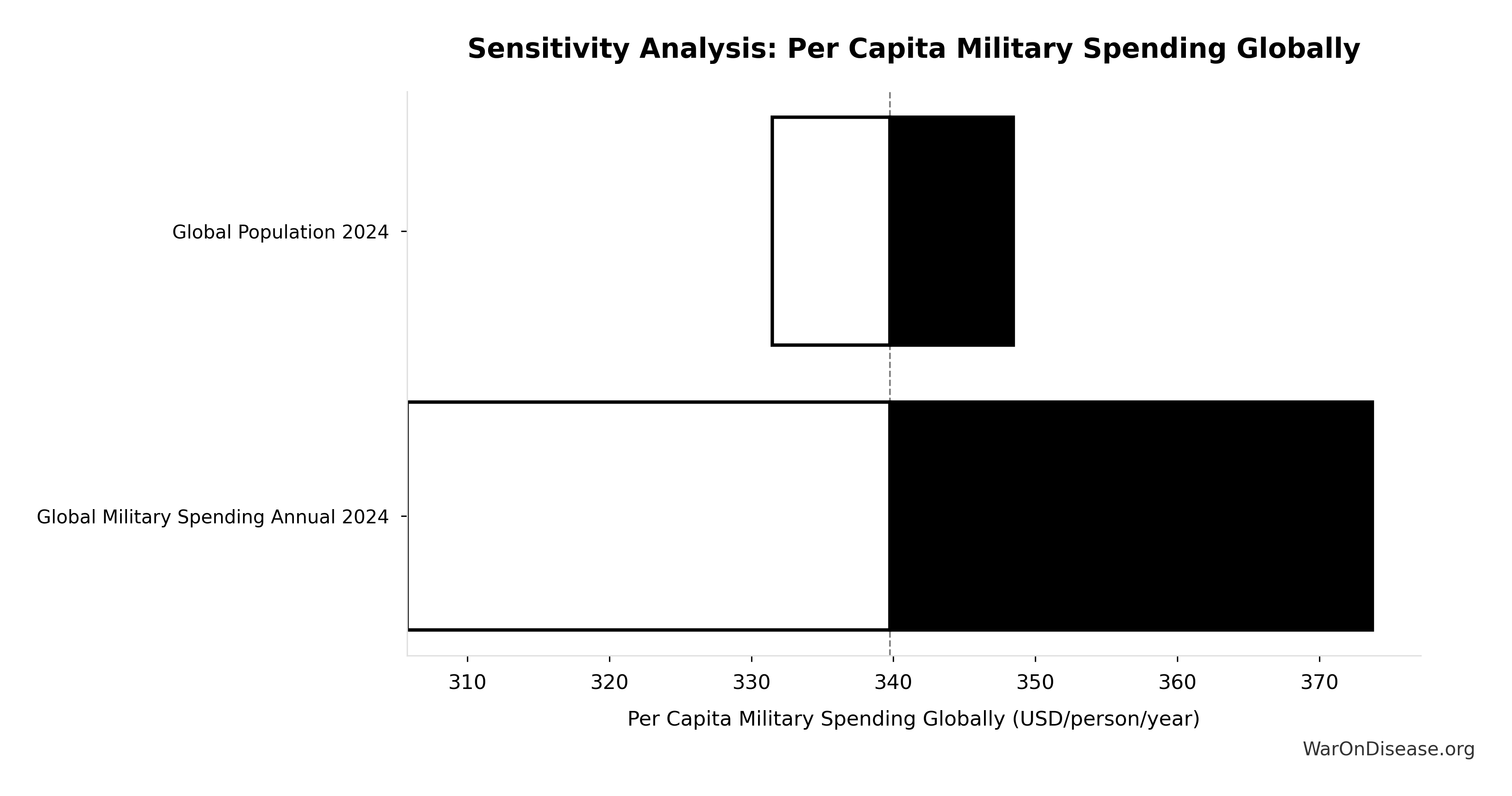
This exceedance probability chart shows the likelihood that Diseases Without Effective Treatment will exceed any given threshold. Higher curves indicate more favorable outcomes with greater certainty.
Ratio of Annual Disease Deaths to 9/11 Terrorism Deaths: 18.4k:1
Note📊 Details
Ratio of annual disease deaths to 9/11 terrorism deaths
Inputs:
- Annual Deaths from All Diseases and Aging Globally 📊: 55 million deaths/year (SE: ±5 million deaths/year)
- Deaths from 9/11 Terrorist Attacks 📊: 3 thousand deaths
\[ \begin{gathered} Ratio_{dis:terror} \\ = \frac{Deaths_{curable,ann}}{Deaths_{9/11}} \\ = \frac{55M}{3{,}000} \\ = 18{,}400 \end{gathered} \]
✓ High confidence
Sensitivity Analysis
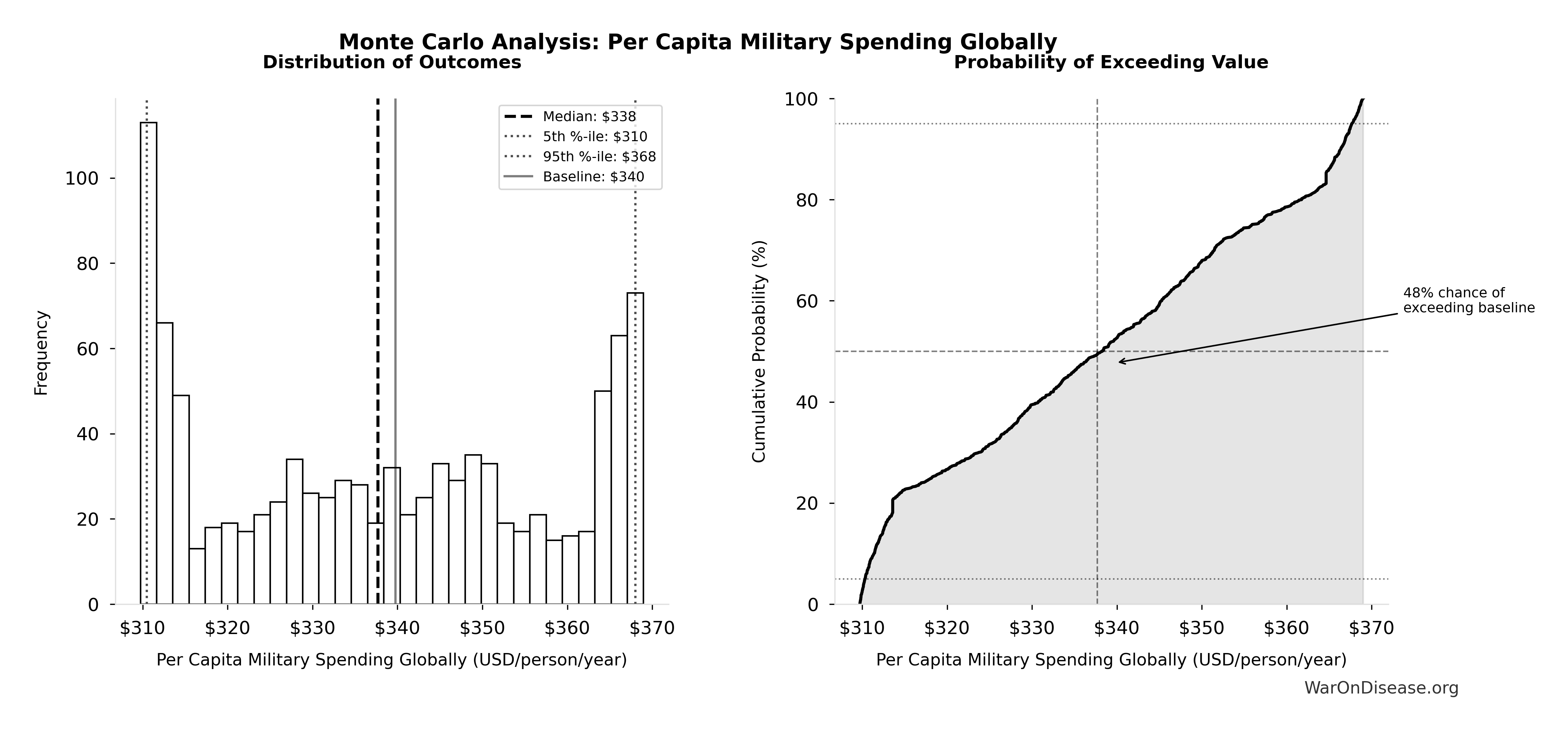
Sensitivity Indices for Ratio of Annual Disease Deaths to 9/11 Terrorism Deaths
Regression-based sensitivity showing which inputs explain the most variance in the output.
| Input Parameter | Sensitivity Coefficient | Interpretation |
|---|---|---|
| Annual Deaths from All Diseases and Aging Globally (deaths/year) | 1.0000 | Strong driver |
Interpretation: Standardized coefficients show the change in output (in SD units) per 1 SD change in input. Values near ±1 indicate strong influence; values exceeding ±1 may occur with correlated inputs.
Monte Carlo Distribution
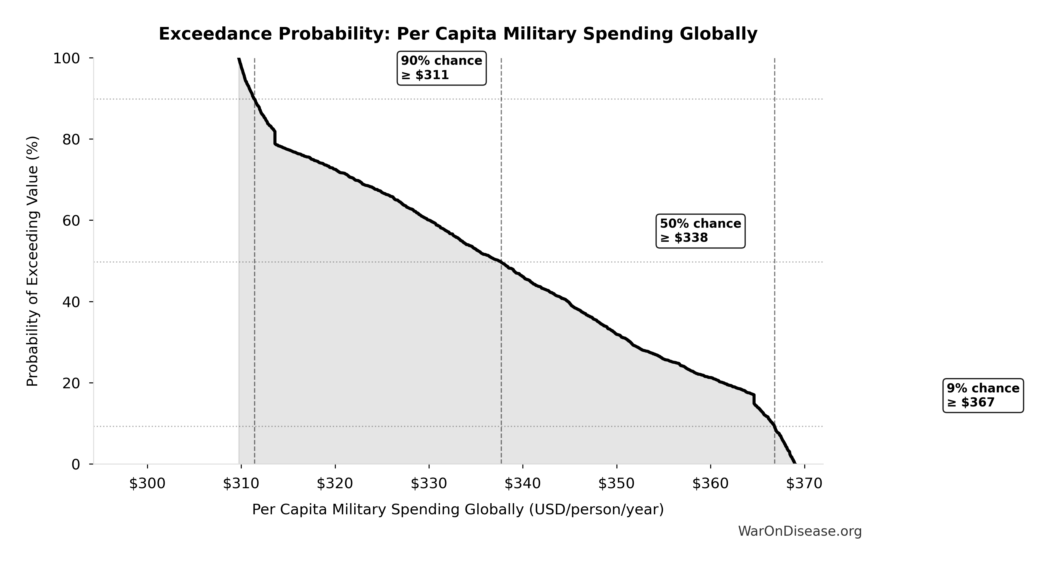
Simulation Results Summary: Ratio of Annual Disease Deaths to 9/11 Terrorism Deaths
| Statistic | Value |
|---|---|
| Baseline (deterministic) | 18.4k:1 |
| Mean (expected value) | 18.3k:1 |
| Median (50th percentile) | 18.3k:1 |
| Standard Deviation | 1.68k:1 |
| 90% Range (5th-95th percentile) | [15.6k:1, 21.1k:1] |
The histogram shows the distribution of Ratio of Annual Disease Deaths to 9/11 Terrorism Deaths across 10,000 Monte Carlo simulations. The CDF (right) shows the probability of the outcome exceeding any given value, which is useful for risk assessment.
Exceedance Probability

This exceedance probability chart shows the likelihood that Ratio of Annual Disease Deaths to 9/11 Terrorism Deaths will exceed any given threshold. Higher curves indicate more favorable outcomes with greater certainty.
Ratio of Annual Disease Deaths to War Deaths: 225:1
Note📊 Details
Ratio of annual disease deaths to war deaths
Inputs:
- Annual Deaths from All Diseases and Aging Globally 📊: 55 million deaths/year (SE: ±5 million deaths/year)
- Total Annual Conflict Deaths Globally 🔢: 245 thousand deaths/year
\[ \begin{gathered} Ratio_{dis:war} \\ = \frac{Deaths_{curable,ann}}{Deaths_{conflict}} \\ = \frac{55M}{245{,}000} \\ = 225 \end{gathered} \] where: \[ \begin{gathered} Deaths_{conflict} \\ = Deaths_{combat} + Deaths_{state} + Deaths_{terror} \\ = 234{,}000 + 2{,}700 + 8{,}300 \\ = 245{,}000 \end{gathered} \] ✓ High confidence
Sensitivity Analysis
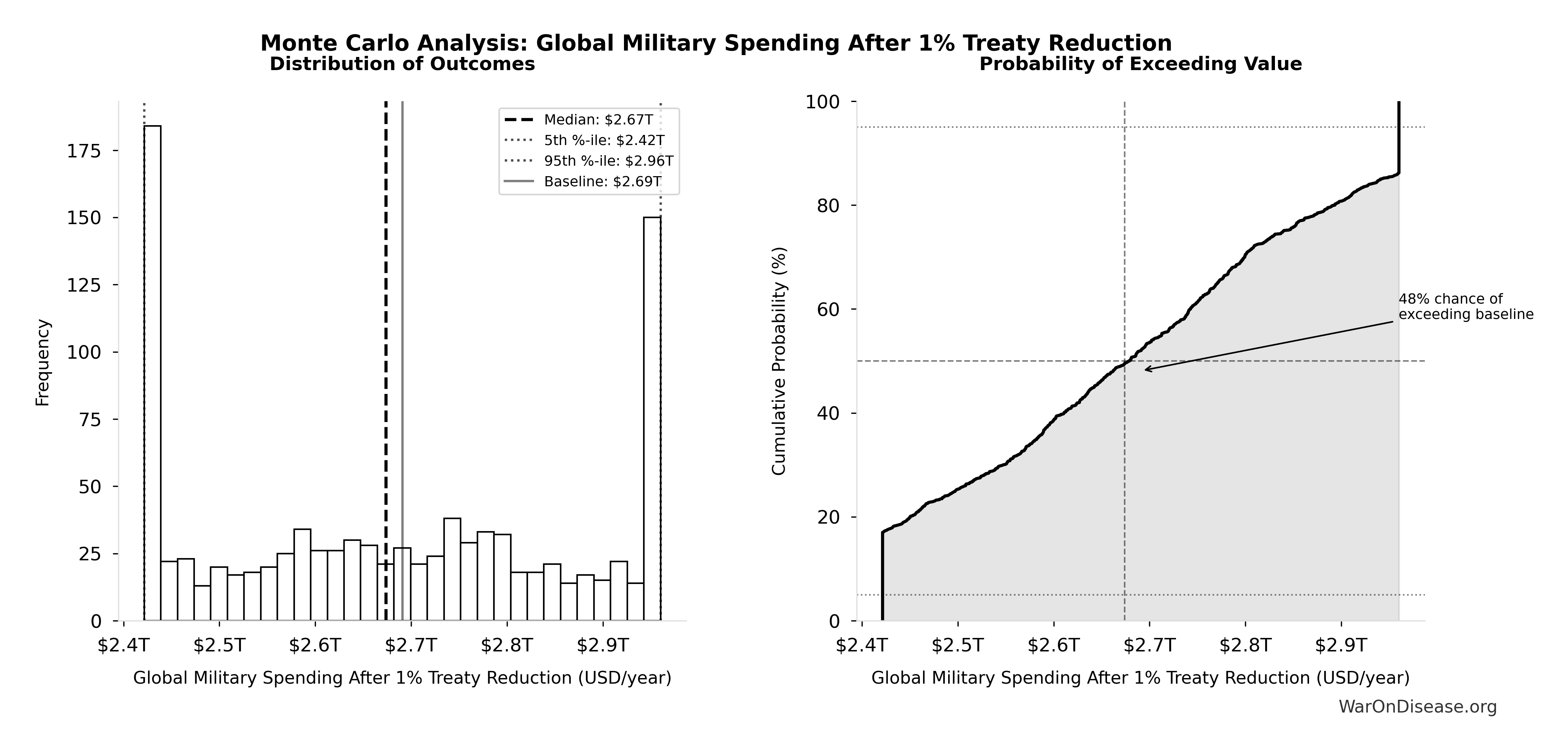
Sensitivity Indices for Ratio of Annual Disease Deaths to War Deaths
Regression-based sensitivity showing which inputs explain the most variance in the output.
| Input Parameter | Sensitivity Coefficient | Interpretation |
|---|---|---|
| Total Annual Conflict Deaths Globally (deaths/year) | -2.9115 | Strong driver |
| Annual Deaths from All Diseases and Aging Globally (deaths/year) | 1.9792 | Strong driver |
Interpretation: Standardized coefficients show the change in output (in SD units) per 1 SD change in input. Values near ±1 indicate strong influence; values exceeding ±1 may occur with correlated inputs.
Monte Carlo Distribution
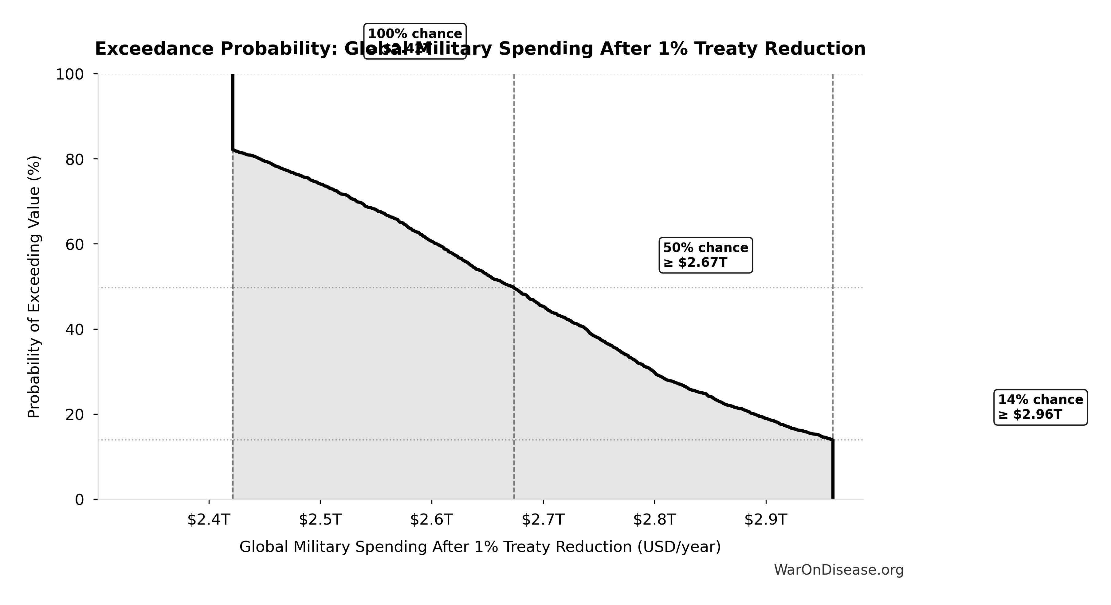
Simulation Results Summary: Ratio of Annual Disease Deaths to War Deaths
| Statistic | Value |
|---|---|
| Baseline (deterministic) | 225:1 |
| Mean (expected value) | 226:1 |
| Median (50th percentile) | 227:1 |
| Standard Deviation | 8.8:1 |
| 90% Range (5th-95th percentile) | [210:1, 239:1] |
The histogram shows the distribution of Ratio of Annual Disease Deaths to War Deaths across 10,000 Monte Carlo simulations. The CDF (right) shows the probability of the outcome exceeding any given value, which is useful for risk assessment.
Exceedance Probability
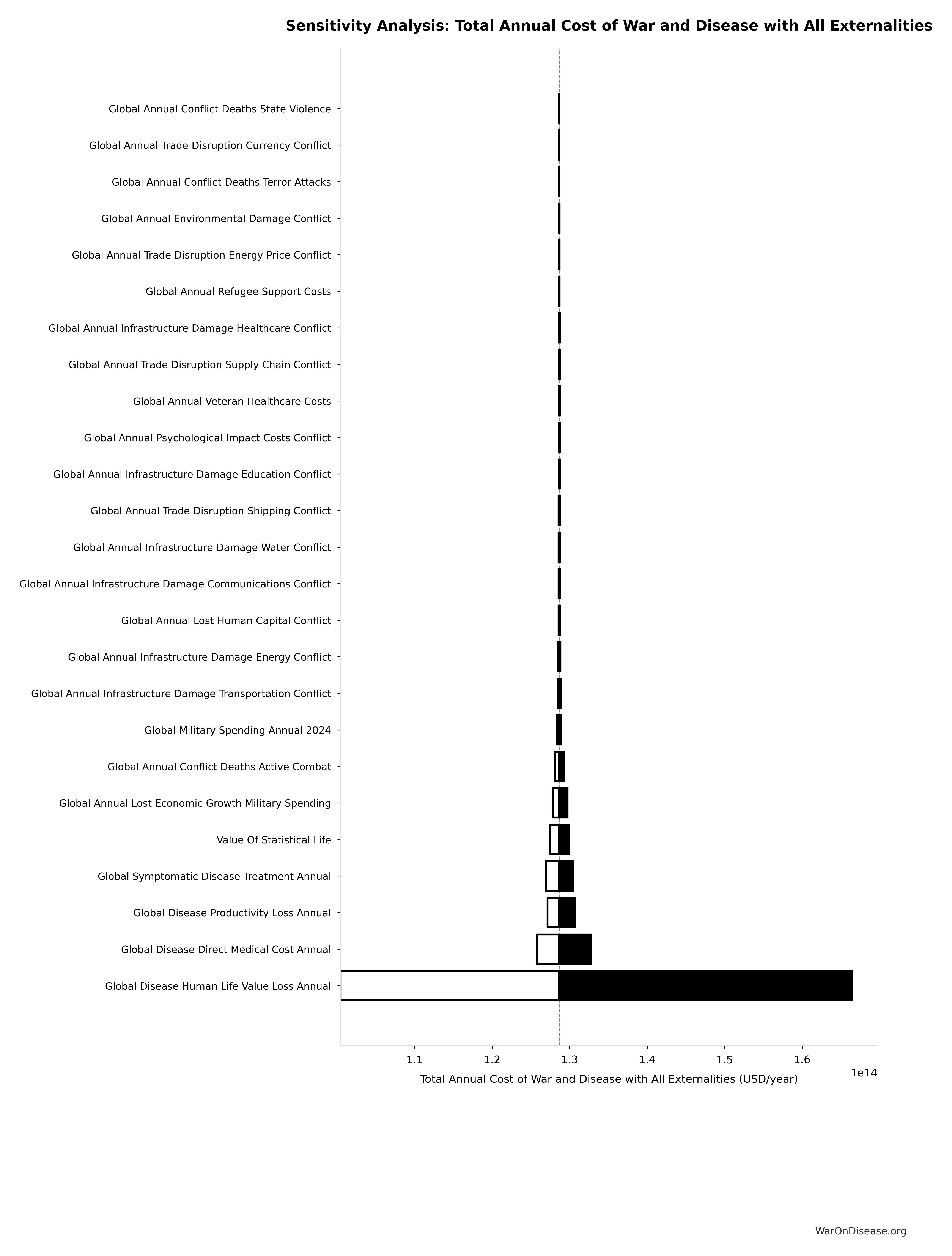
This exceedance probability chart shows the likelihood that Ratio of Annual Disease Deaths to War Deaths will exceed any given threshold. Higher curves indicate more favorable outcomes with greater certainty.
Drug Cost Increase: 1980s to Current: 13.4x
Note📊 Details
Drug development cost increase from 1980s to current
Inputs:
- Drug Development Cost (1980s) 📊: $194M (95% CI: $146M - $242M)
- Pharma Drug Development Cost (Current System) 📊: $2.6B (95% CI: $1.5B - $4B)
\[ \begin{gathered} k_{cost,80s} \\ = \frac{Cost_{dev,curr}}{Cost_{dev,80s}} \\ = \frac{\$2.6B}{\$194M} \\ = 13.4 \end{gathered} \]
Methodology:23
✓ High confidence
Sensitivity Analysis
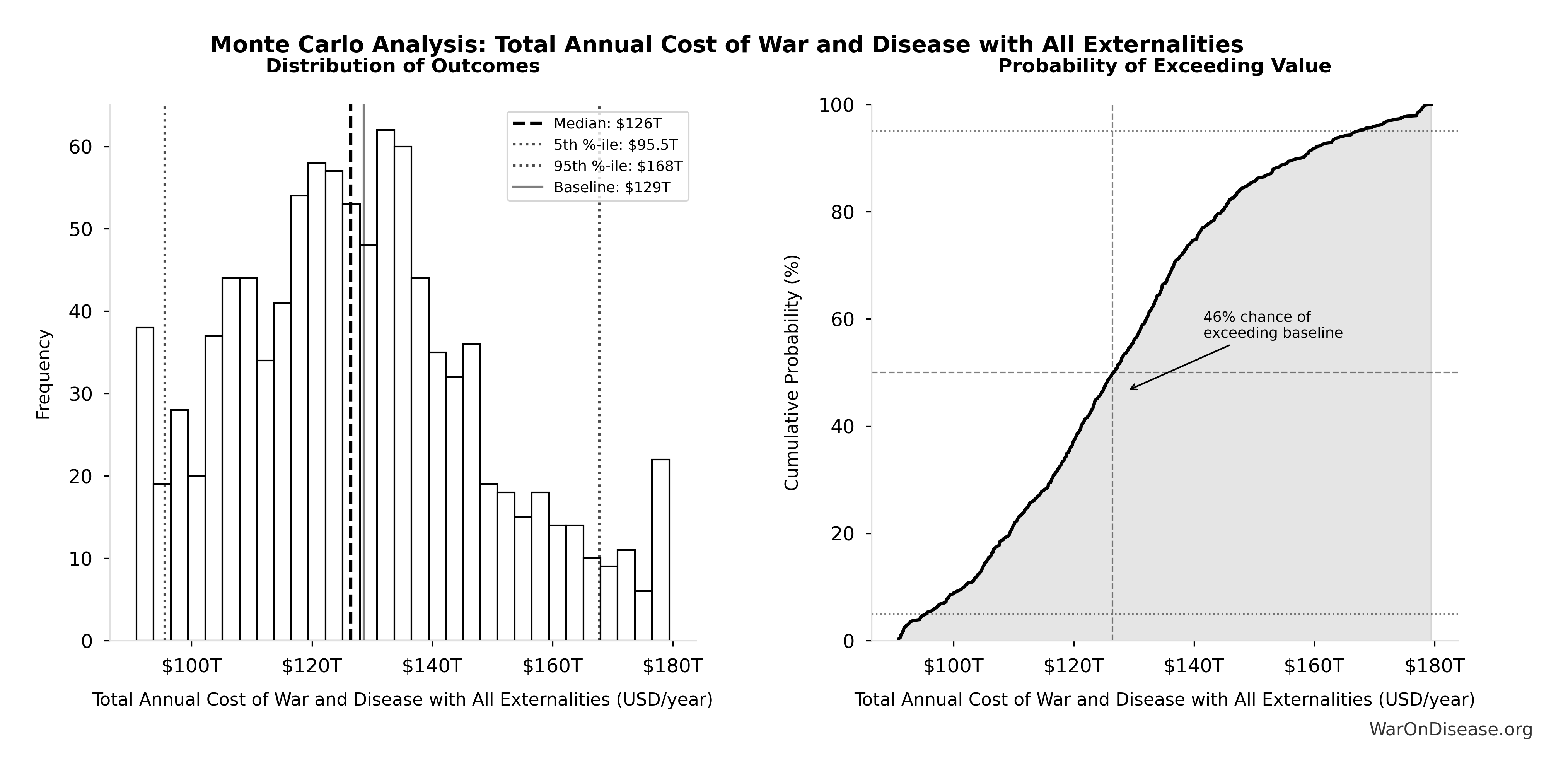
Sensitivity Indices for Drug Cost Increase: 1980s to Current
Regression-based sensitivity showing which inputs explain the most variance in the output.
| Input Parameter | Sensitivity Coefficient | Interpretation |
|---|---|---|
| Pharma Drug Development Cost (Current System) (USD) | 1.6909 | Strong driver |
| Drug Development Cost (1980s) (USD) | -0.7048 | Strong driver |
Interpretation: Standardized coefficients show the change in output (in SD units) per 1 SD change in input. Values near ±1 indicate strong influence; values exceeding ±1 may occur with correlated inputs.
Monte Carlo Distribution
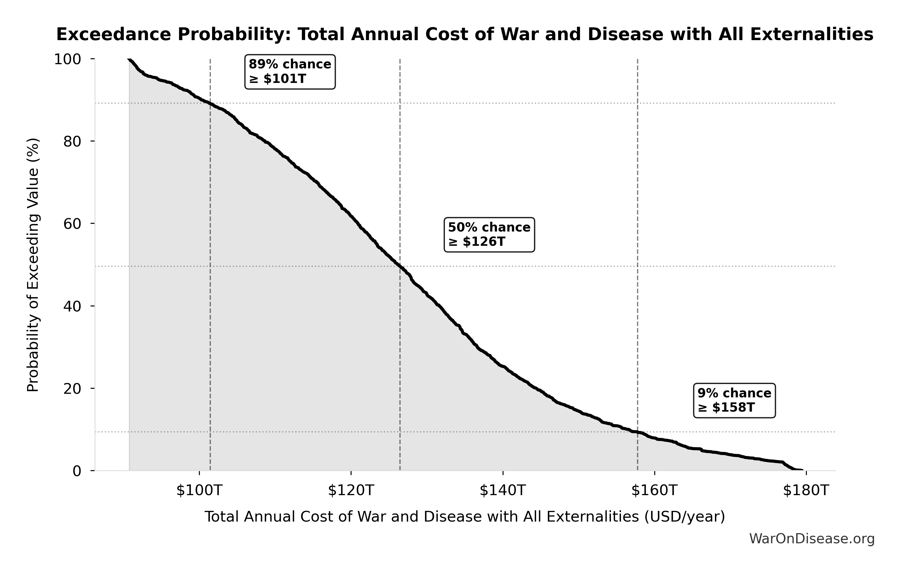
Simulation Results Summary: Drug Cost Increase: 1980s to Current
| Statistic | Value |
|---|---|
| Baseline (deterministic) | 13.4x |
| Mean (expected value) | 13.3x |
| Median (50th percentile) | 13.3x |
| Standard Deviation | 0.915x |
| 90% Range (5th-95th percentile) | [11.9x, 14.7x] |
The histogram shows the distribution of Drug Cost Increase: 1980s to Current across 10,000 Monte Carlo simulations. The CDF (right) shows the probability of the outcome exceeding any given value, which is useful for risk assessment.
Exceedance Probability
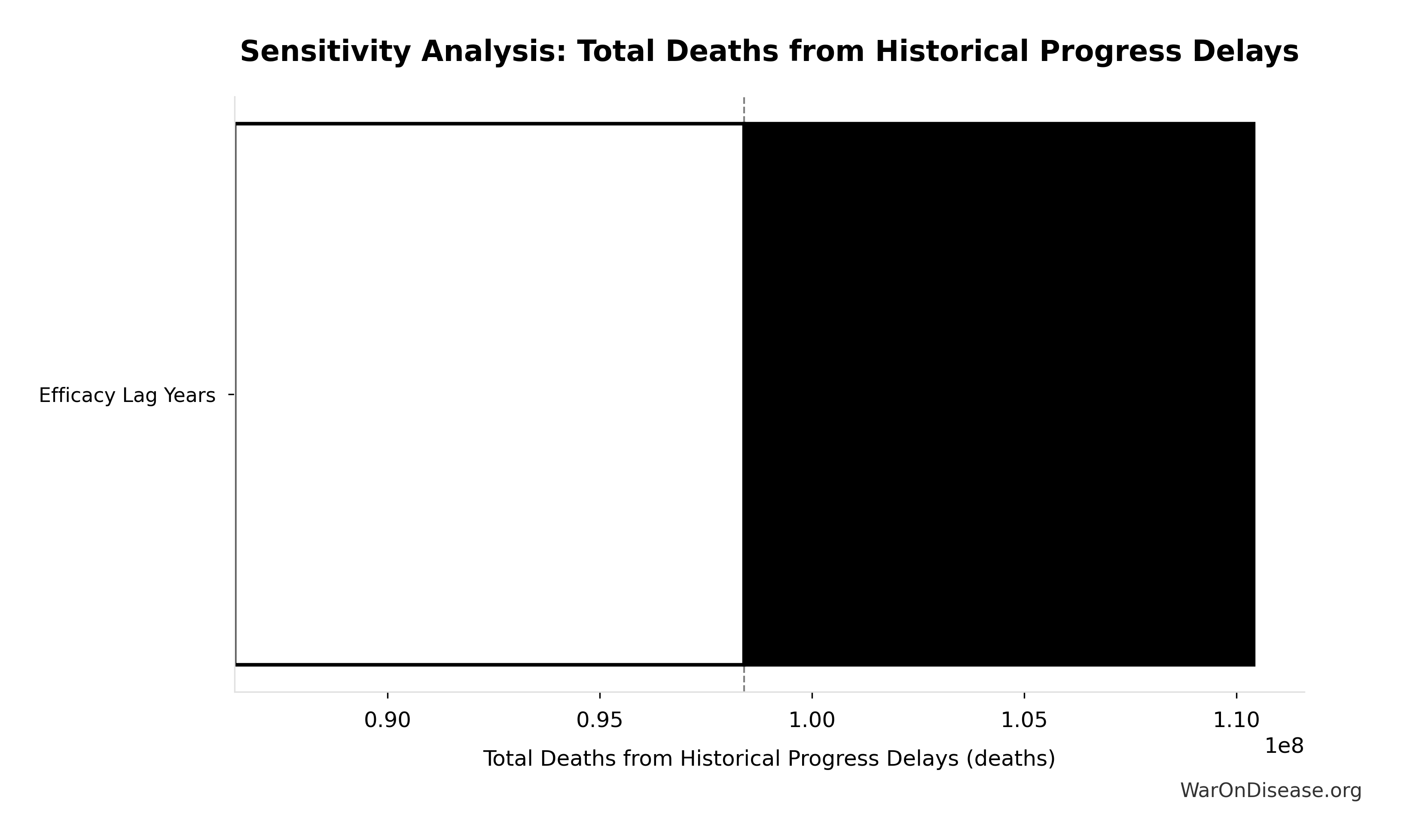
This exceedance probability chart shows the likelihood that Drug Cost Increase: 1980s to Current will exceed any given threshold. Higher curves indicate more favorable outcomes with greater certainty.
Drug Cost Increase: Pre-1962 to Current: 105x
Note📊 Details
Drug development cost increase from pre-1962 to current
Inputs:
- Pharma Drug Development Cost (Current System) 📊: $2.6B (95% CI: $1.5B - $4B)
- Pre-1962 Drug Development Cost (2024 Dollars) 📊: $24.7M (95% CI: $19.5M - $30M)
\[ \begin{gathered} k_{cost,pre62} \\ = \frac{Cost_{dev,curr}}{Cost_{pre62,24}} \\ = \frac{\$2.6B}{\$24.7M} \\ = 105 \end{gathered} \]
Methodology:85
✓ High confidence
Sensitivity Analysis
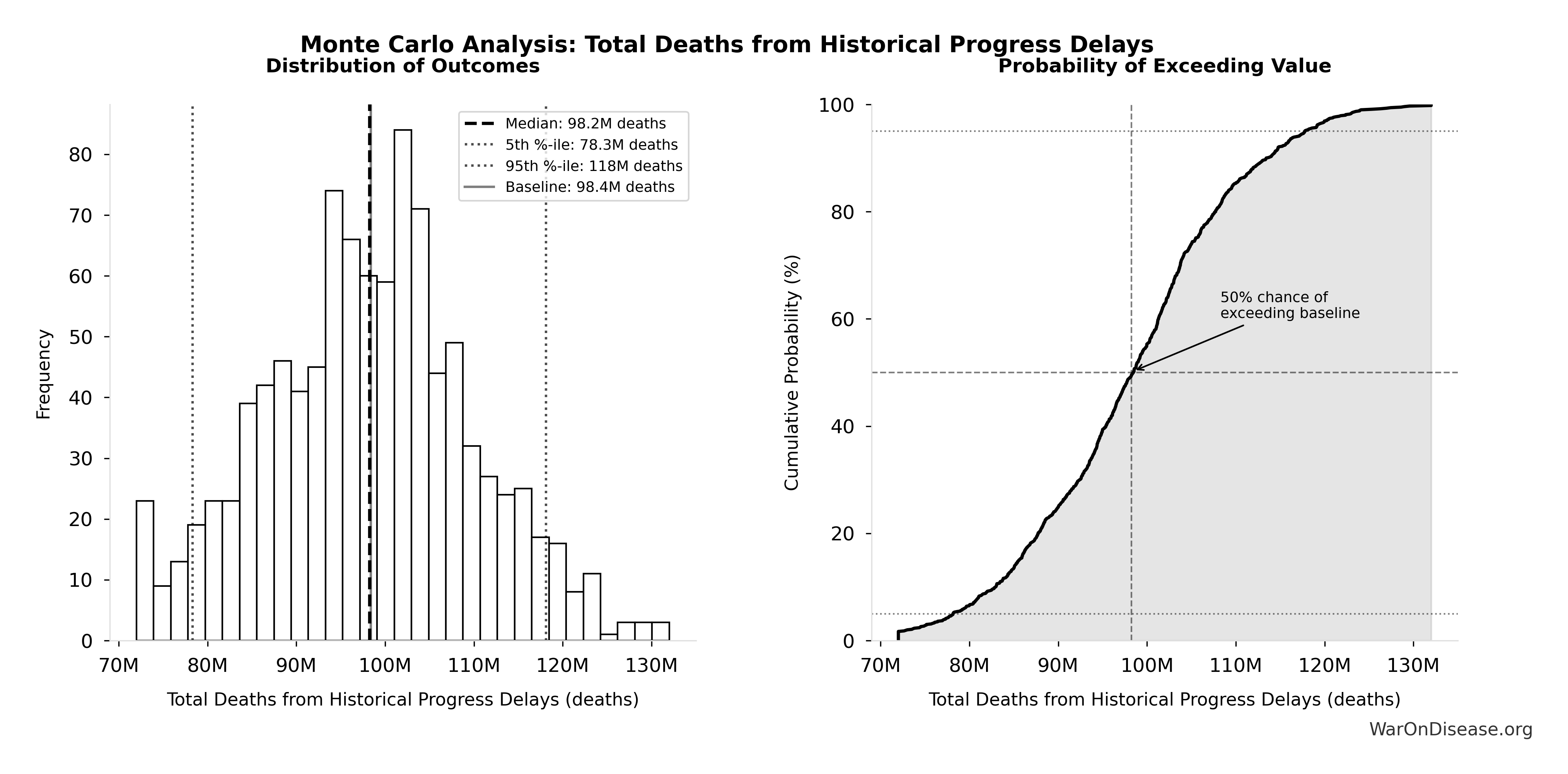
Sensitivity Indices for Drug Cost Increase: Pre-1962 to Current
Regression-based sensitivity showing which inputs explain the most variance in the output.
| Input Parameter | Sensitivity Coefficient | Interpretation |
|---|---|---|
| Pharma Drug Development Cost (Current System) (USD) | 1.3110 | Strong driver |
| Pre-1962 Drug Development Cost (2024 Dollars) (USD) | -0.3181 | Moderate driver |
Interpretation: Standardized coefficients show the change in output (in SD units) per 1 SD change in input. Values near ±1 indicate strong influence; values exceeding ±1 may occur with correlated inputs.
Monte Carlo Distribution
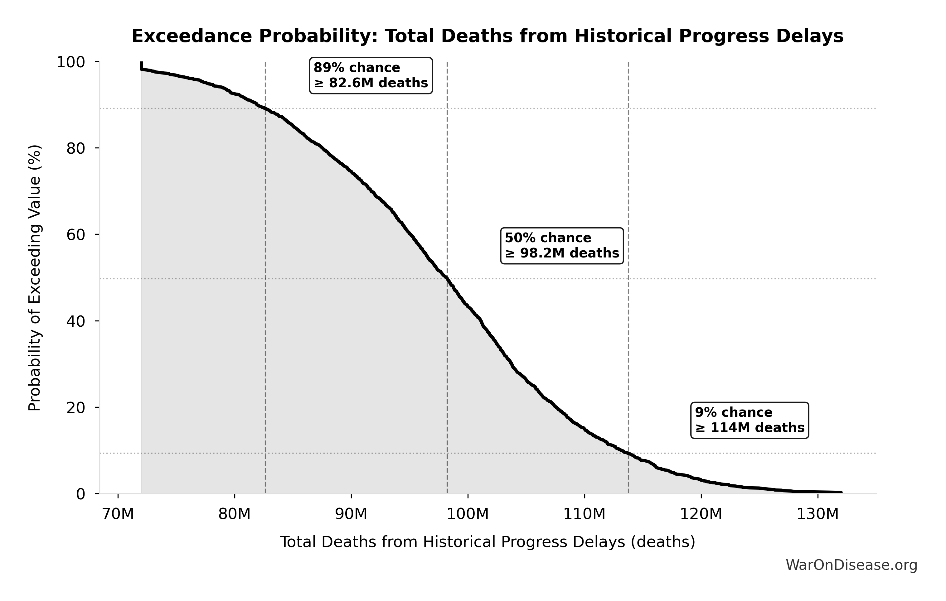
Simulation Results Summary: Drug Cost Increase: Pre-1962 to Current
| Statistic | Value |
|---|---|
| Baseline (deterministic) | 105x |
| Mean (expected value) | 104x |
| Median (50th percentile) | 104x |
| Standard Deviation | 9.03x |
| 90% Range (5th-95th percentile) | [90.6x, 119x] |
The histogram shows the distribution of Drug Cost Increase: Pre-1962 to Current across 10,000 Monte Carlo simulations. The CDF (right) shows the probability of the outcome exceeding any given value, which is useful for risk assessment.
Exceedance Probability
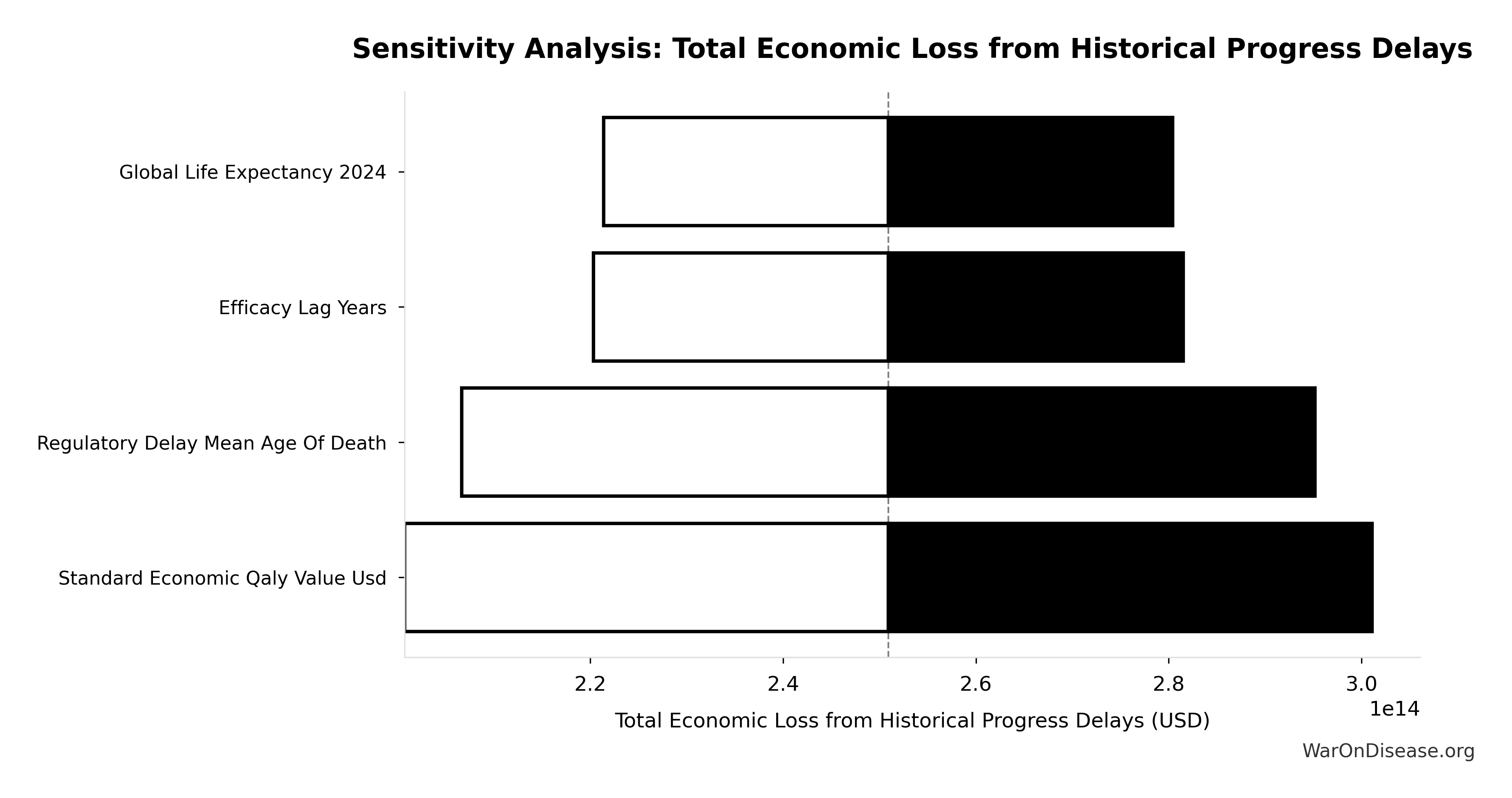
This exceedance probability chart shows the likelihood that Drug Cost Increase: Pre-1962 to Current will exceed any given threshold. Higher curves indicate more favorable outcomes with greater certainty.
Possible Drug-Disease Combinations: 9.5 million combinations
Note📊 Details
Total possible drug-disease combinations using existing safe compounds
Inputs:
- Safe Compounds Available for Testing: 9.5 thousand compounds (95% CI: 7 thousand compounds - 12 thousand compounds)
- Trial-Relevant Diseases: 1 thousand diseases (95% CI: 800 diseases - 1.2 thousand diseases)
\[ \begin{gathered} N_{combos} \\ = N_{safe} \times N_{diseases,trial} \\ = 9{,}500 \times 1{,}000 \\ = 9.5M \end{gathered} \]
✓ High confidence
Sensitivity Analysis
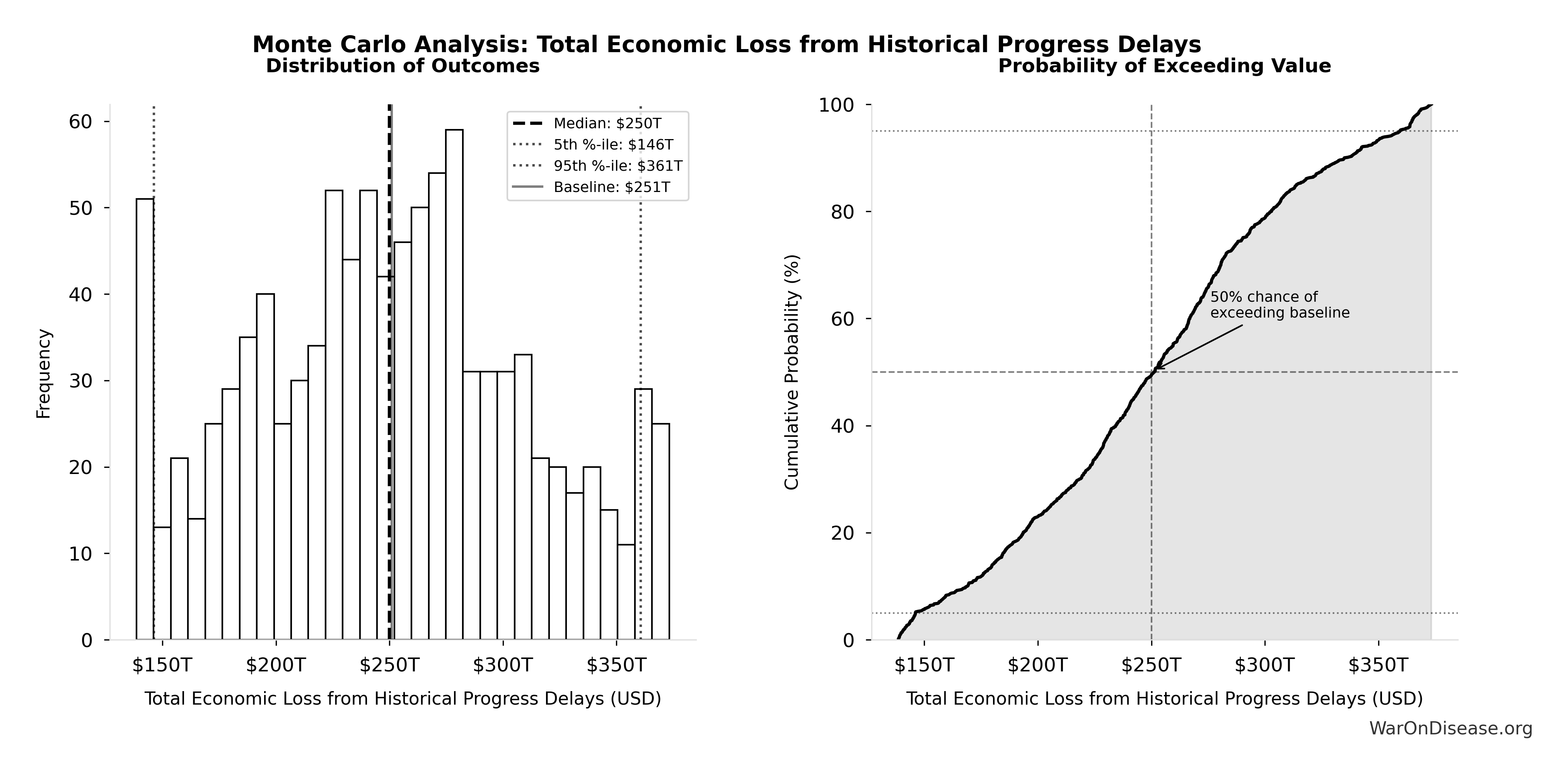
Therapeutic Frontier Exploration Ratio: 0.342%
Note📊 Details
Fraction of possible drug-disease space actually tested (<1%)
Inputs:
- Tested Drug-Disease Relationships: 32.5 thousand relationships (95% CI: 15 thousand relationships - 50 thousand relationships)
- Possible Drug-Disease Combinations 🔢: 9.5 million combinations
\[ \begin{gathered} Ratio_{explore} \\ = \frac{N_{tested}}{N_{combos}} \\ = \frac{32{,}500}{9.5M} \\ = 0.342\% \end{gathered} \] where: \[ \begin{gathered} N_{combos} \\ = N_{safe} \times N_{diseases,trial} \\ = 9{,}500 \times 1{,}000 \\ = 9.5M \end{gathered} \] ✓ High confidence
Sensitivity Analysis
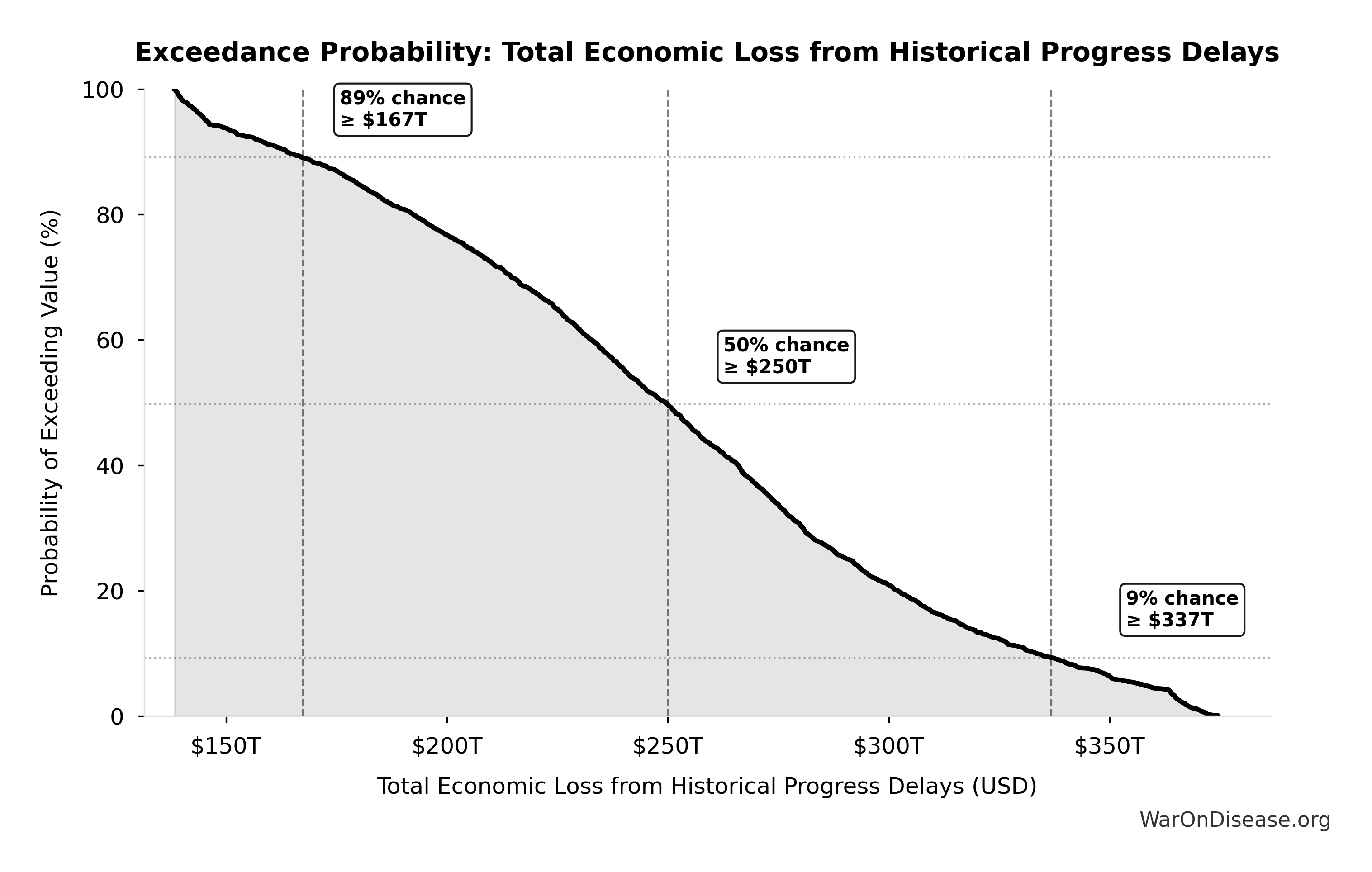
Sensitivity Indices for Therapeutic Frontier Exploration Ratio
Regression-based sensitivity showing which inputs explain the most variance in the output.
| Input Parameter | Sensitivity Coefficient | Interpretation |
|---|---|---|
| Tested Drug-Disease Relationships (relationships) | 1.0000 | Strong driver |
Interpretation: Standardized coefficients show the change in output (in SD units) per 1 SD change in input. Values near ±1 indicate strong influence; values exceeding ±1 may occur with correlated inputs.
Monte Carlo Distribution
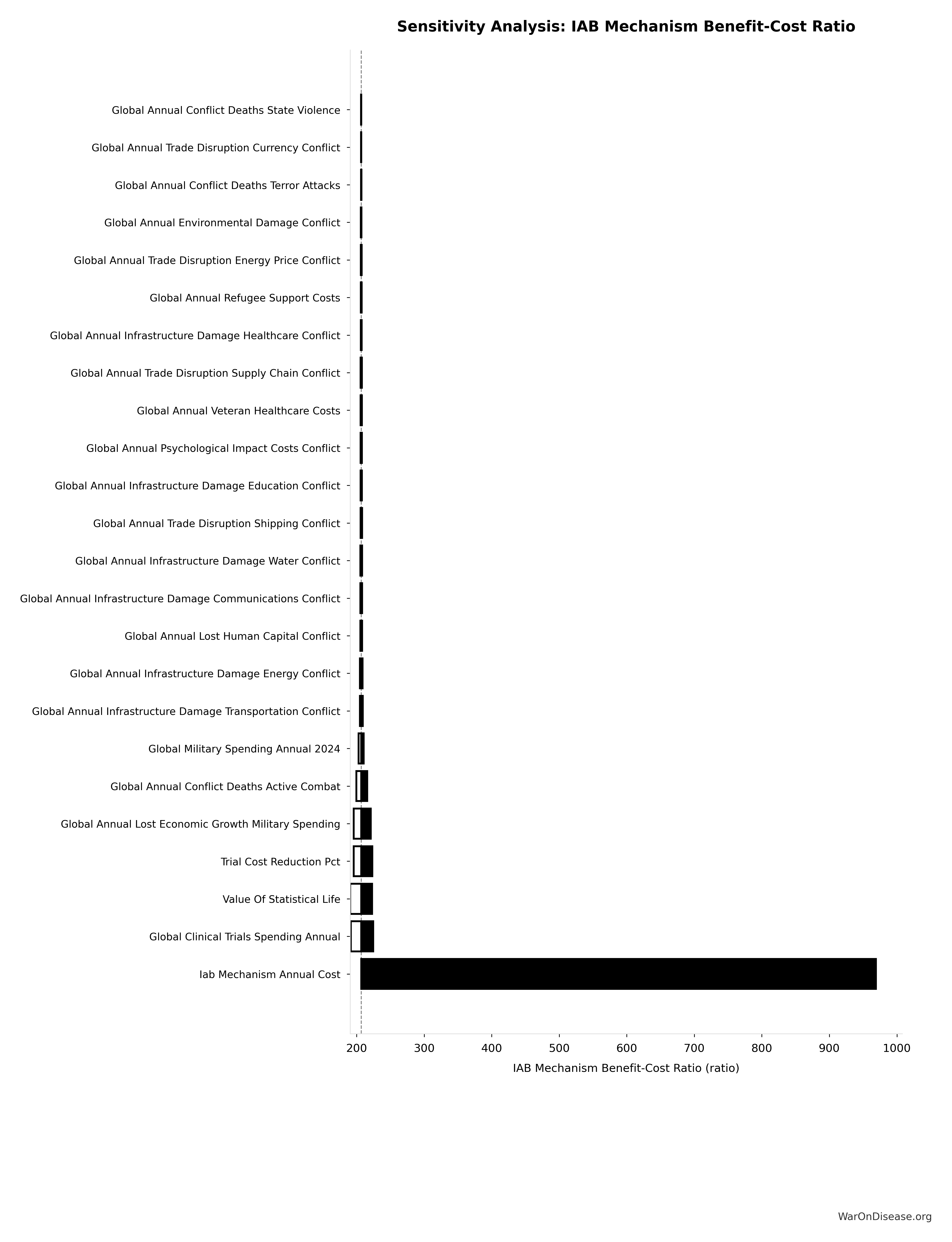
Simulation Results Summary: Therapeutic Frontier Exploration Ratio
| Statistic | Value |
|---|---|
| Baseline (deterministic) | 0.342% |
| Mean (expected value) | 0.339% |
| Median (50th percentile) | 0.329% |
| Standard Deviation | 0.0868% |
| 90% Range (5th-95th percentile) | [0.21%, 0.514%] |
The histogram shows the distribution of Therapeutic Frontier Exploration Ratio across 10,000 Monte Carlo simulations. The CDF (right) shows the probability of the outcome exceeding any given value, which is useful for risk assessment.
Exceedance Probability
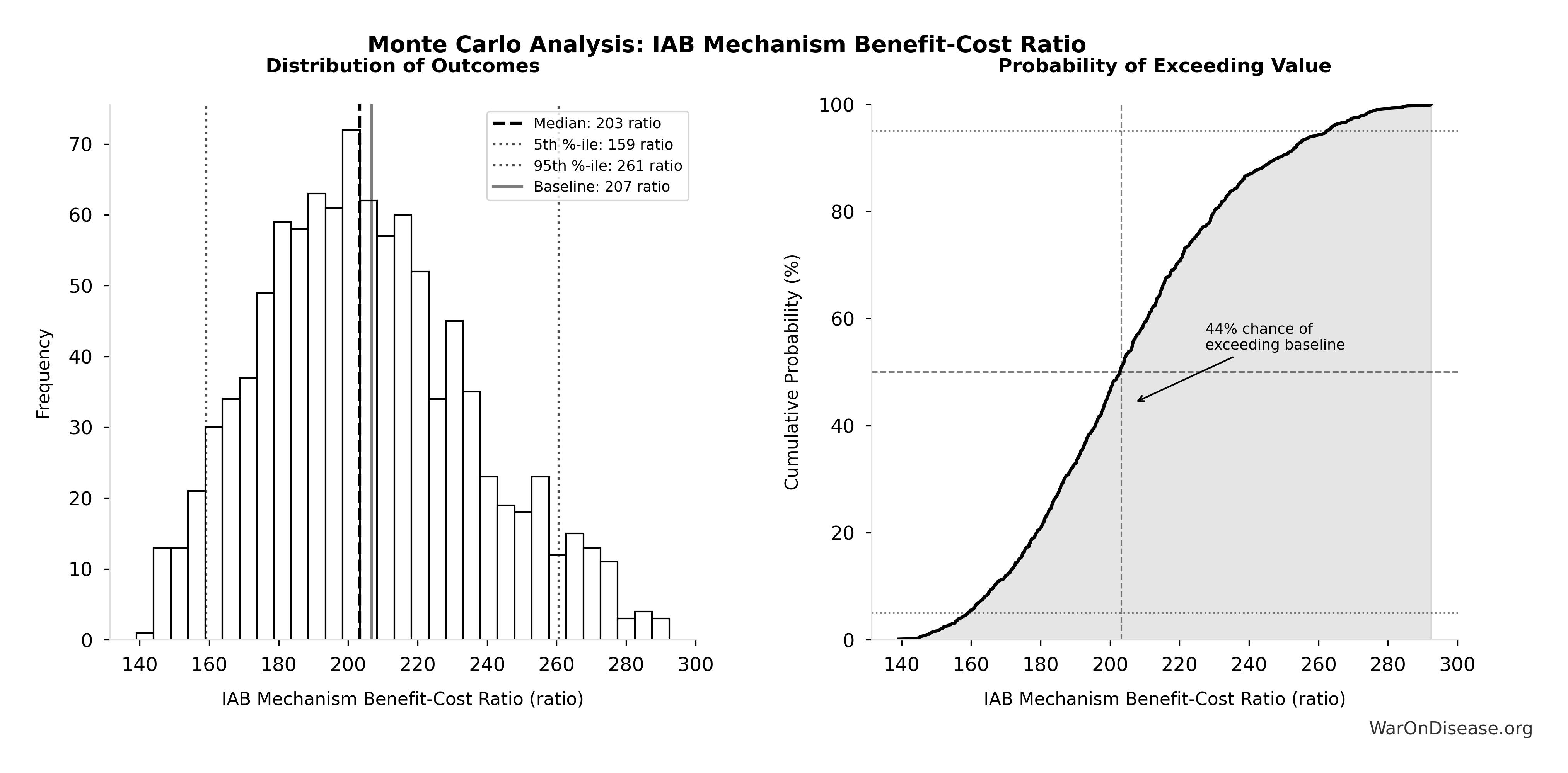
This exceedance probability chart shows the likelihood that Therapeutic Frontier Exploration Ratio will exceed any given threshold. Higher curves indicate more favorable outcomes with greater certainty.
Total Annual Conflict Deaths Globally: 245 thousand deaths/year
Note📊 Details
Total annual conflict deaths globally (sum of combat, terror, state violence)
Inputs:
- Annual Deaths from Active Combat Worldwide 📊: 234 thousand deaths/year (95% CI: 180 thousand deaths/year - 300 thousand deaths/year)
- Annual Deaths from State Violence 📊: 2.7 thousand deaths/year (95% CI: 1.5 thousand deaths/year - 5 thousand deaths/year)
- Annual Deaths from Terror Attacks Globally 📊: 8.3 thousand deaths/year (95% CI: 6 thousand deaths/year - 12 thousand deaths/year)
\[ \begin{gathered} Deaths_{conflict} \\ = Deaths_{combat} + Deaths_{state} + Deaths_{terror} \\ = 234{,}000 + 2{,}700 + 8{,}300 \\ = 245{,}000 \end{gathered} \]
✓ High confidence
Sensitivity Analysis
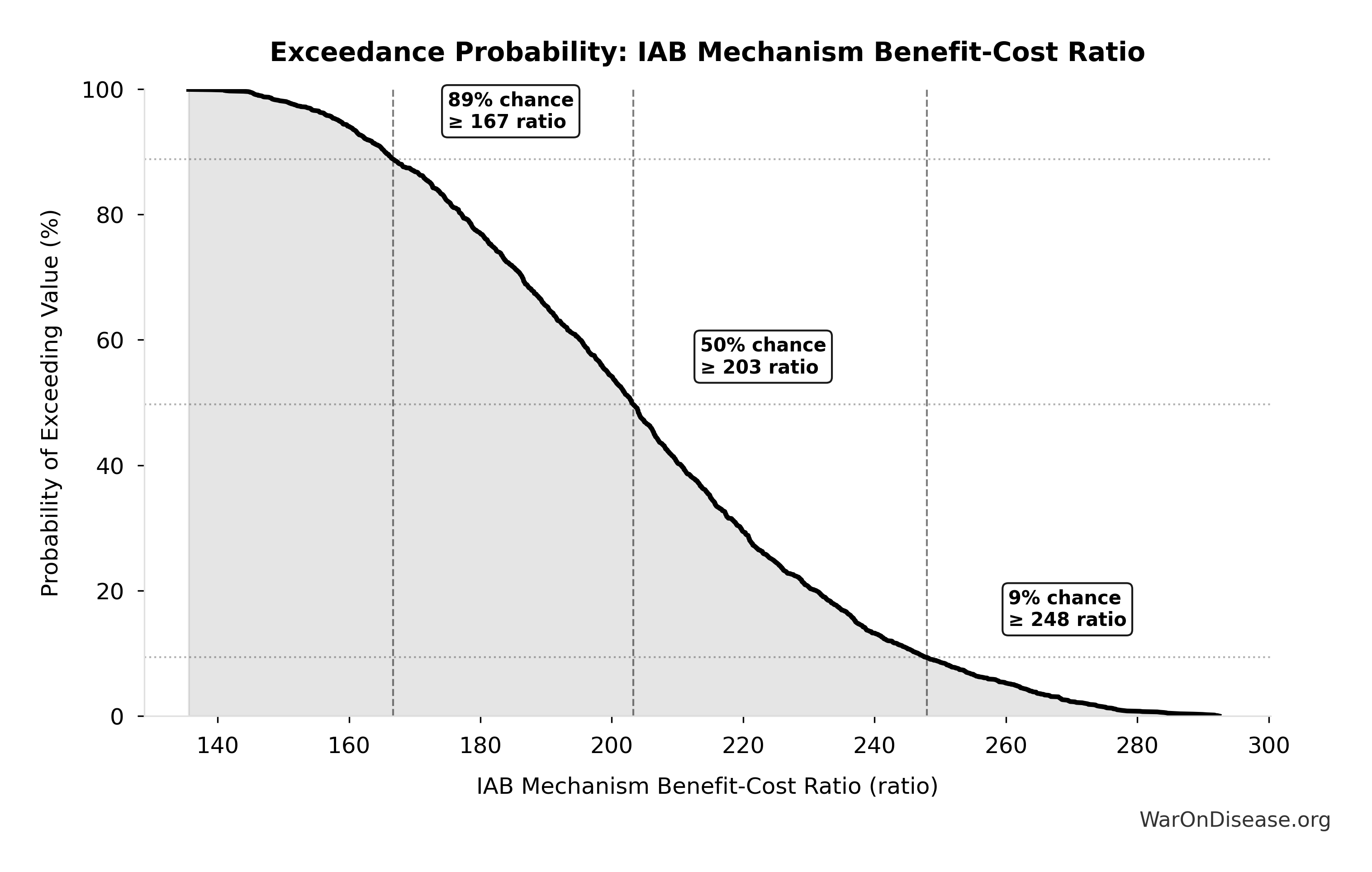
Sensitivity Indices for Total Annual Conflict Deaths Globally
Regression-based sensitivity showing which inputs explain the most variance in the output.
| Input Parameter | Sensitivity Coefficient | Interpretation |
|---|---|---|
| Annual Deaths from Active Combat Worldwide (deaths/year) | 0.9276 | Strong driver |
| Annual Deaths from Terror Attacks Globally (deaths/year) | 0.0461 | Minimal effect |
| Annual Deaths from State Violence (deaths/year) | 0.0266 | Minimal effect |
Interpretation: Standardized coefficients show the change in output (in SD units) per 1 SD change in input. Values near ±1 indicate strong influence; values exceeding ±1 may occur with correlated inputs.
Monte Carlo Distribution

Simulation Results Summary: Total Annual Conflict Deaths Globally
| Statistic | Value |
|---|---|
| Baseline (deterministic) | 245 thousand |
| Mean (expected value) | 244 thousand |
| Median (50th percentile) | 242 thousand |
| Standard Deviation | 31.5 thousand |
| 90% Range (5th-95th percentile) | [194 thousand, 302 thousand] |
The histogram shows the distribution of Total Annual Conflict Deaths Globally across 10,000 Monte Carlo simulations. The CDF (right) shows the probability of the outcome exceeding any given value, which is useful for risk assessment.
Exceedance Probability

This exceedance probability chart shows the likelihood that Total Annual Conflict Deaths Globally will exceed any given threshold. Higher curves indicate more favorable outcomes with greater certainty.
Total Annual Cost of War Worldwide: $11.4T
Note📊 Details
Total annual cost of war worldwide (direct + indirect costs)
Inputs:
- Total Annual Direct War Costs 🔢: $7.66T
- Total Annual Indirect War Costs 🔢: $3.7T
\[ \begin{gathered} Cost_{war,total} \\ = Cost_{war,direct} + Cost_{war,indirect} \\ = \$7.66T + \$3.7T \\ = \$11.4T \end{gathered} \] where: \[ \begin{gathered} Cost_{war,direct} \\ = Loss_{life,conflict} + Damage_{infra,total} \\ + Disruption_{trade} + Spending_{mil} \\ = \$2.45T + \$1.88T + \$616B + \$2.72T \\ = \$7.66T \end{gathered} \] where: \[ \begin{gathered} Loss_{life,conflict} \\ = Cost_{combat,human} + Cost_{state,human} \\ + Cost_{terror,human} \\ = \$2.34T + \$27B + \$83B \\ = \$2.45T \end{gathered} \] where: \[ \begin{gathered} Cost_{combat,human} \\ = Deaths_{combat} \times VSL \\ = 234{,}000 \times \$10M \\ = \$2.34T \end{gathered} \] where: \[ \begin{gathered} Cost_{state,human} \\ = Deaths_{state} \times VSL \\ = 2{,}700 \times \$10M \\ = \$27B \end{gathered} \] where: \[ \begin{gathered} Cost_{terror,human} \\ = Deaths_{terror} \times VSL \\ = 8{,}300 \times \$10M \\ = \$83B \end{gathered} \] where: \[ \begin{gathered} Damage_{infra,total} \\ = Damage_{comms} + Damage_{edu} + Damage_{energy} \\ + Damage_{health} + Damage_{transport} + Damage_{water} \\ = \$298B + \$234B + \$422B + \$166B + \$487B + \$268B \\ = \$1.88T \end{gathered} \] where: \[ \begin{gathered} Disruption_{trade} \\ = Disruption_{currency} + Disruption_{energy} \\ + Disruption_{shipping} + Disruption_{supply} \\ = \$57.4B + \$125B + \$247B + \$187B \\ = \$616B \end{gathered} \] where: \[ \begin{gathered} Cost_{war,indirect} \\ = Damage_{env} + Loss_{growth,mil} + Loss_{capital,conflict} \\ + Cost_{psych} + Cost_{refugee} + Cost_{vet} \\ = \$100B + \$2.72T + \$300B + \$232B + \$150B + \$200B \\ = \$3.7T \end{gathered} \] ✓ High confidence
Sensitivity Analysis
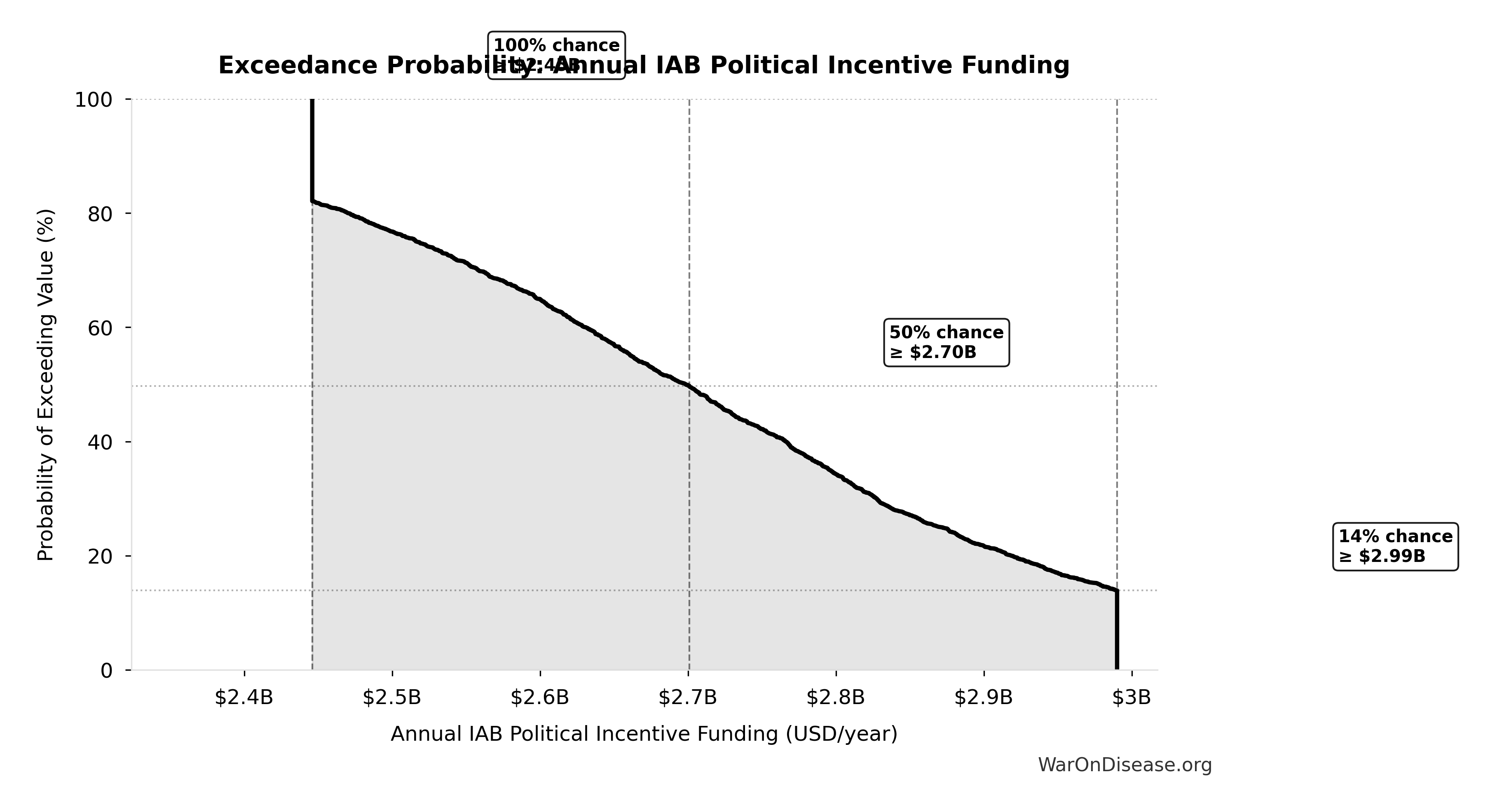
Sensitivity Indices for Total Annual Cost of War Worldwide
Regression-based sensitivity showing which inputs explain the most variance in the output.
| Input Parameter | Sensitivity Coefficient | Interpretation |
|---|---|---|
| Total Annual Direct War Costs (USD/year) | 0.6553 | Strong driver |
| Total Annual Indirect War Costs (USD/year) | 0.4150 | Moderate driver |
Interpretation: Standardized coefficients show the change in output (in SD units) per 1 SD change in input. Values near ±1 indicate strong influence; values exceeding ±1 may occur with correlated inputs.
Monte Carlo Distribution

Simulation Results Summary: Total Annual Cost of War Worldwide
| Statistic | Value |
|---|---|
| Baseline (deterministic) | $11.4T |
| Mean (expected value) | $11.3T |
| Median (50th percentile) | $11.2T |
| Standard Deviation | $1.51T |
| 90% Range (5th-95th percentile) | [$9.01T, $14.1T] |
The histogram shows the distribution of Total Annual Cost of War Worldwide across 10,000 Monte Carlo simulations. The CDF (right) shows the probability of the outcome exceeding any given value, which is useful for risk assessment.
Exceedance Probability
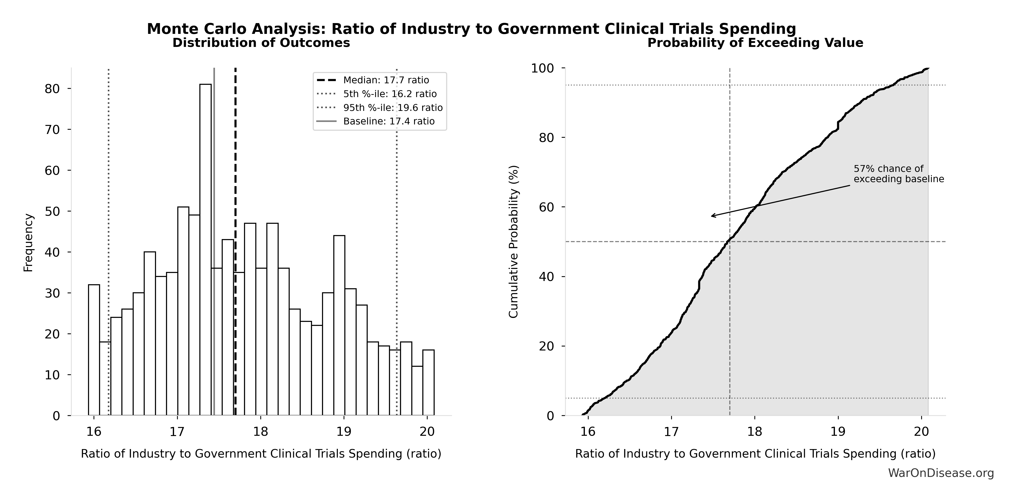
This exceedance probability chart shows the likelihood that Total Annual Cost of War Worldwide will exceed any given threshold. Higher curves indicate more favorable outcomes with greater certainty.
Annual Cost of Combat Deaths: $2.34T
Note📊 Details
Annual cost of combat deaths (deaths × VSL)
Inputs:
- Annual Deaths from Active Combat Worldwide 📊: 234 thousand deaths/year (95% CI: 180 thousand deaths/year - 300 thousand deaths/year)
- Value of Statistical Life 📊: $10M (95% CI: $5M - $15M)
\[ \begin{gathered} Cost_{combat,human} \\ = Deaths_{combat} \times VSL \\ = 234{,}000 \times \$10M \\ = \$2.34T \end{gathered} \]
✓ High confidence
Sensitivity Analysis
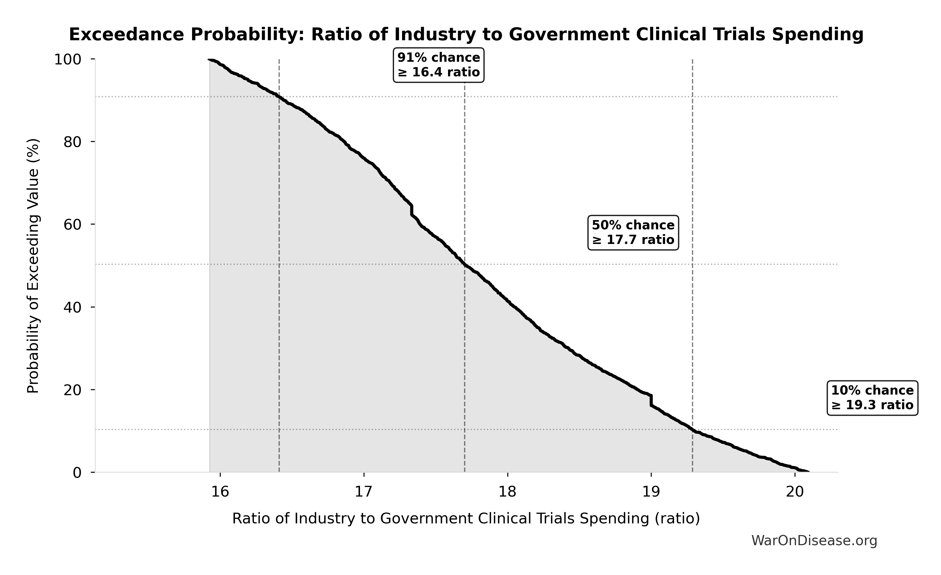
Sensitivity Indices for Annual Cost of Combat Deaths
Regression-based sensitivity showing which inputs explain the most variance in the output.
| Input Parameter | Sensitivity Coefficient | Interpretation |
|---|---|---|
| Value of Statistical Life (USD) | 0.9096 | Strong driver |
| Annual Deaths from Active Combat Worldwide (deaths/year) | 0.4115 | Moderate driver |
Interpretation: Standardized coefficients show the change in output (in SD units) per 1 SD change in input. Values near ±1 indicate strong influence; values exceeding ±1 may occur with correlated inputs.
Monte Carlo Distribution
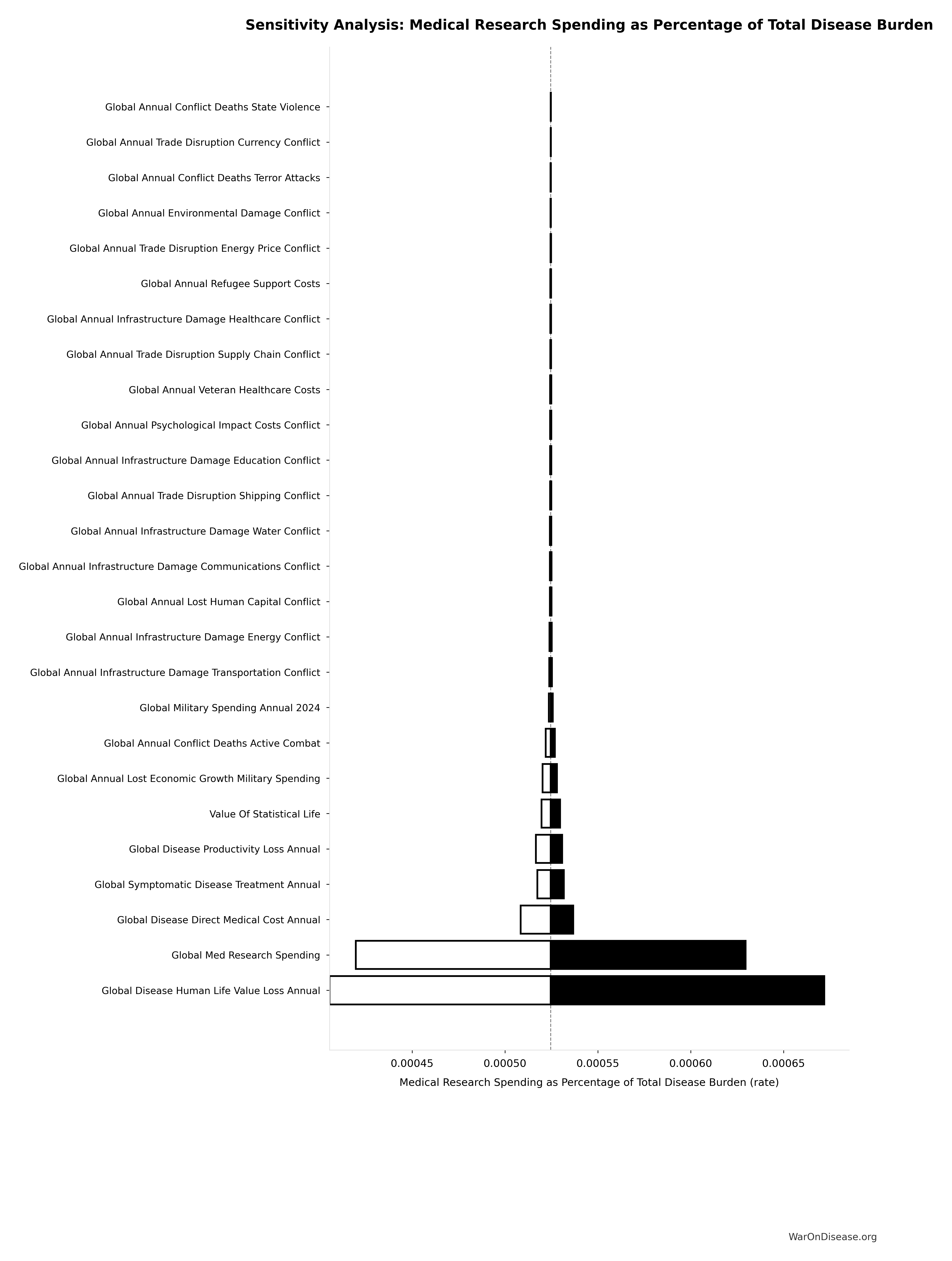
Simulation Results Summary: Annual Cost of Combat Deaths
| Statistic | Value |
|---|---|
| Baseline (deterministic) | $2.34T |
| Mean (expected value) | $2.31T |
| Median (50th percentile) | $2.24T |
| Standard Deviation | $703B |
| 90% Range (5th-95th percentile) | [$1.25T, $3.57T] |
The histogram shows the distribution of Annual Cost of Combat Deaths across 10,000 Monte Carlo simulations. The CDF (right) shows the probability of the outcome exceeding any given value, which is useful for risk assessment.
Exceedance Probability
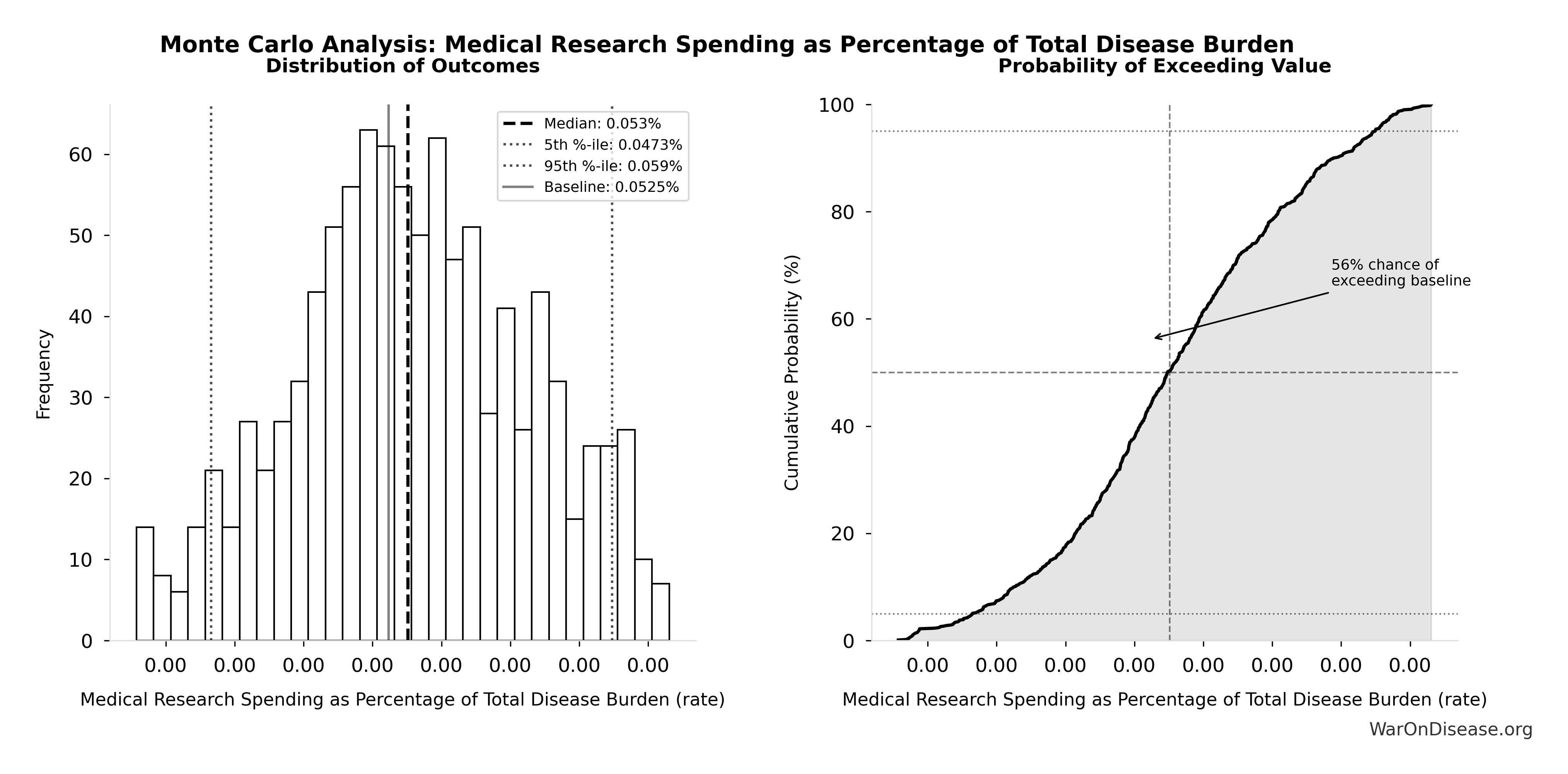
This exceedance probability chart shows the likelihood that Annual Cost of Combat Deaths will exceed any given threshold. Higher curves indicate more favorable outcomes with greater certainty.
Annual Cost of State Violence Deaths: $27B
Note📊 Details
Annual cost of state violence deaths (deaths × VSL)
Inputs:
- Annual Deaths from State Violence 📊: 2.7 thousand deaths/year (95% CI: 1.5 thousand deaths/year - 5 thousand deaths/year)
- Value of Statistical Life 📊: $10M (95% CI: $5M - $15M)
\[ \begin{gathered} Cost_{state,human} \\ = Deaths_{state} \times VSL \\ = 2{,}700 \times \$10M \\ = \$27B \end{gathered} \]
✓ High confidence
Sensitivity Analysis
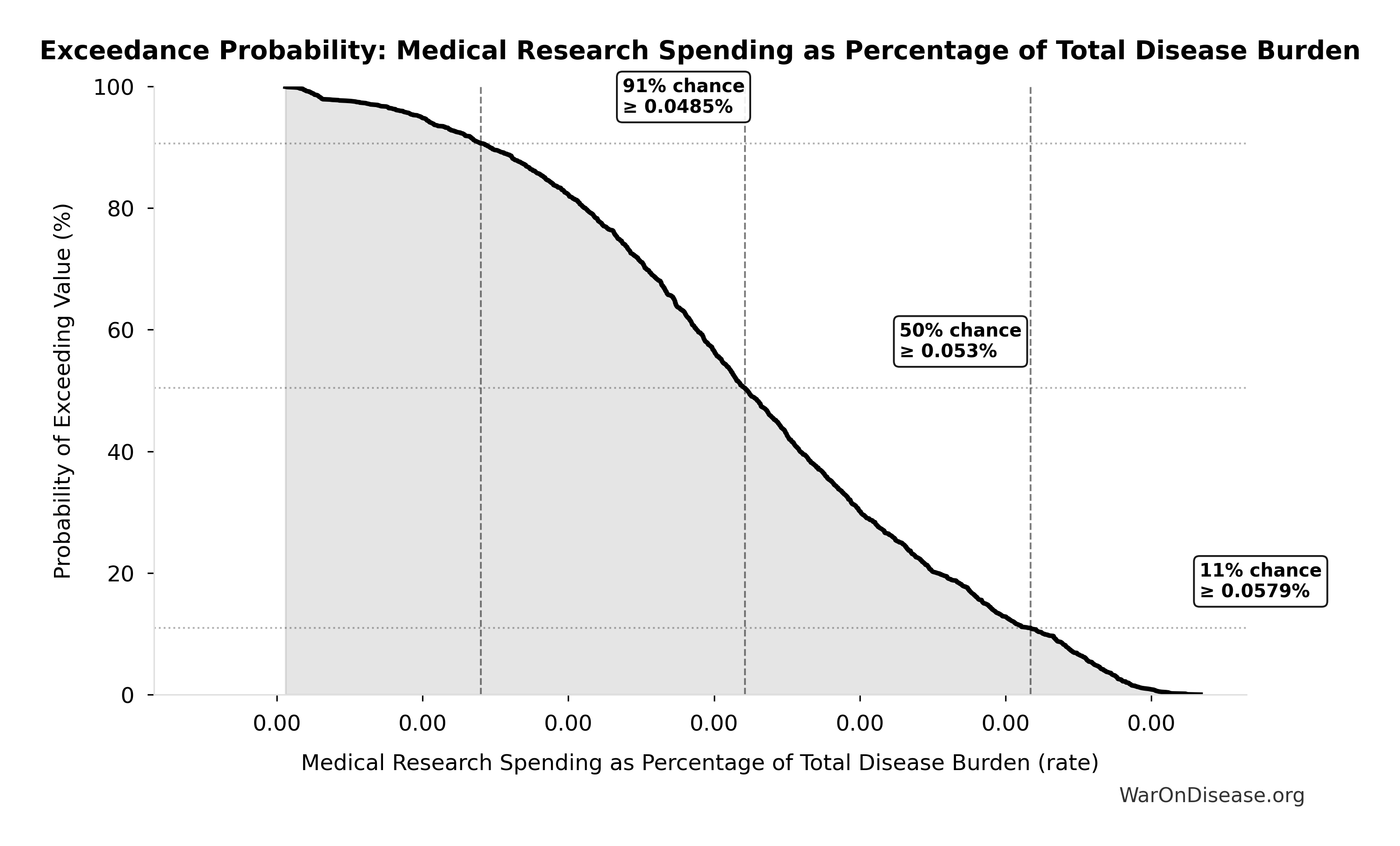
Sensitivity Indices for Annual Cost of State Violence Deaths
Regression-based sensitivity showing which inputs explain the most variance in the output.
| Input Parameter | Sensitivity Coefficient | Interpretation |
|---|---|---|
| Annual Deaths from State Violence (deaths/year) | 0.7358 | Strong driver |
| Value of Statistical Life (USD) | 0.6553 | Strong driver |
Interpretation: Standardized coefficients show the change in output (in SD units) per 1 SD change in input. Values near ±1 indicate strong influence; values exceeding ±1 may occur with correlated inputs.
Monte Carlo Distribution
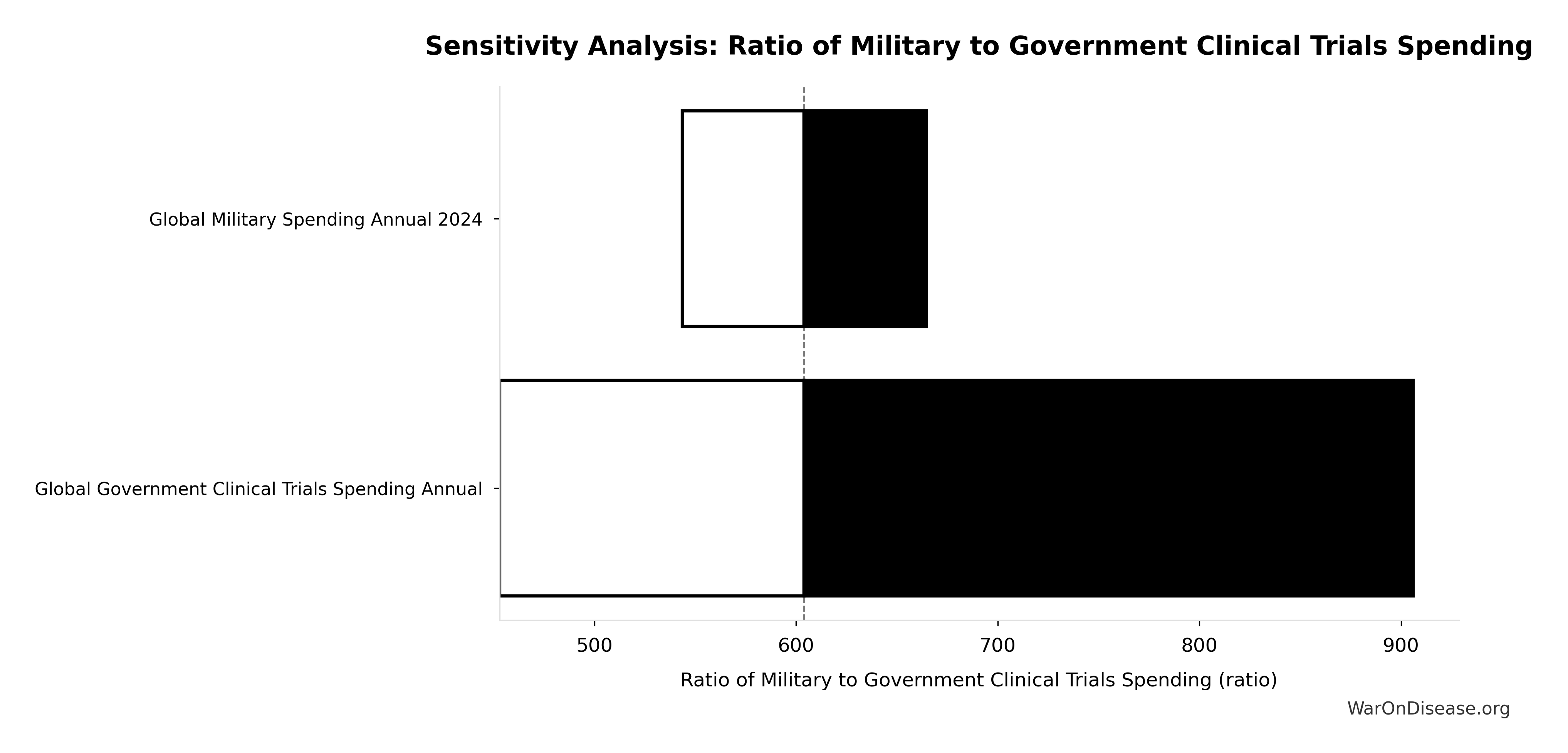
Simulation Results Summary: Annual Cost of State Violence Deaths
| Statistic | Value |
|---|---|
| Baseline (deterministic) | $27B |
| Mean (expected value) | $26.6B |
| Median (50th percentile) | $24.5B |
| Standard Deviation | $11.3B |
| 90% Range (5th-95th percentile) | [$12B, $48.4B] |
The histogram shows the distribution of Annual Cost of State Violence Deaths across 10,000 Monte Carlo simulations. The CDF (right) shows the probability of the outcome exceeding any given value, which is useful for risk assessment.
Exceedance Probability
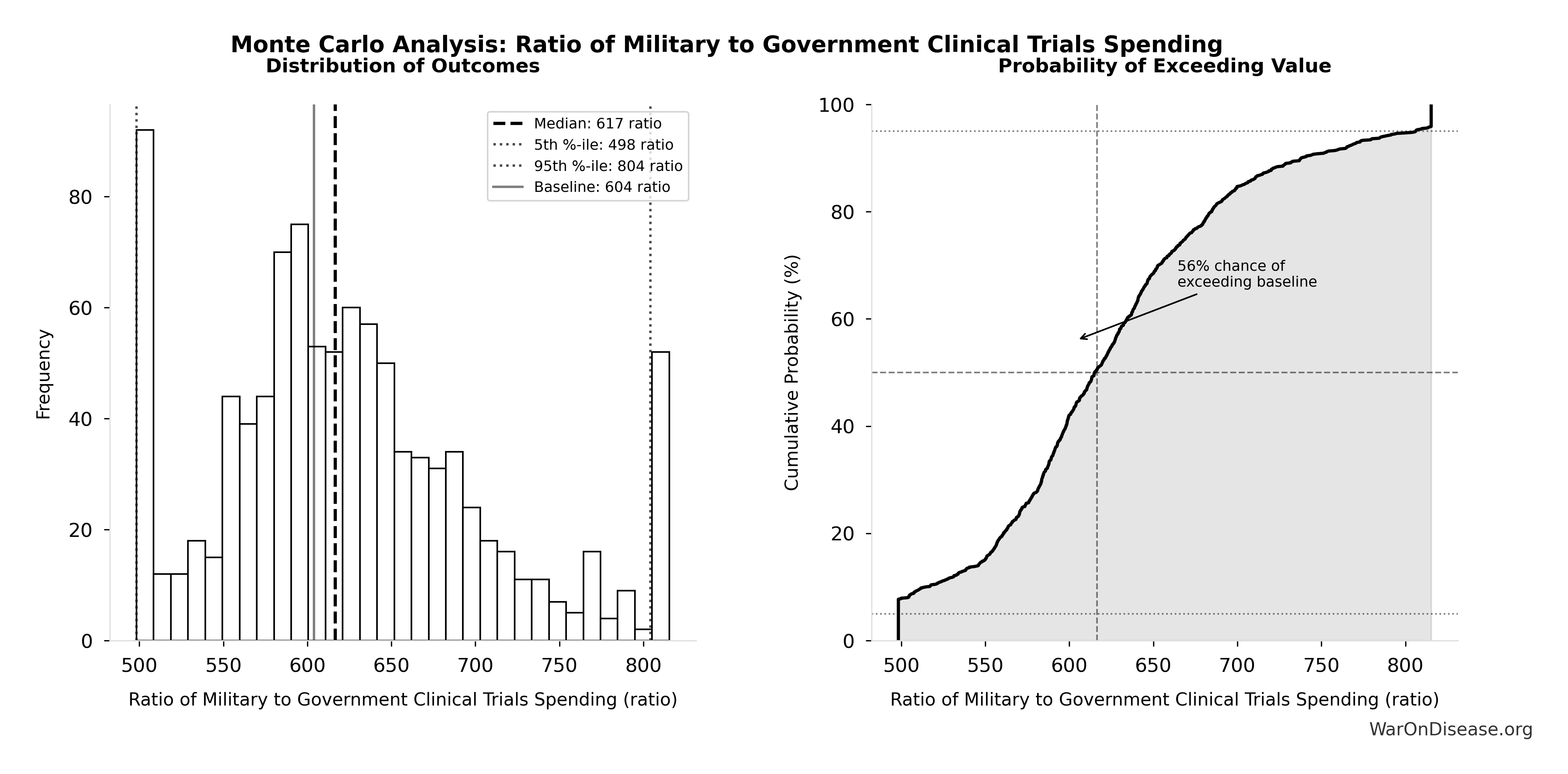
This exceedance probability chart shows the likelihood that Annual Cost of State Violence Deaths will exceed any given threshold. Higher curves indicate more favorable outcomes with greater certainty.
Annual Cost of Terror Deaths: $83B
Note📊 Details
Annual cost of terror deaths (deaths × VSL)
Inputs:
- Annual Deaths from Terror Attacks Globally 📊: 8.3 thousand deaths/year (95% CI: 6 thousand deaths/year - 12 thousand deaths/year)
- Value of Statistical Life 📊: $10M (95% CI: $5M - $15M)
\[ \begin{gathered} Cost_{terror,human} \\ = Deaths_{terror} \times VSL \\ = 8{,}300 \times \$10M \\ = \$83B \end{gathered} \]
✓ High confidence
Sensitivity Analysis
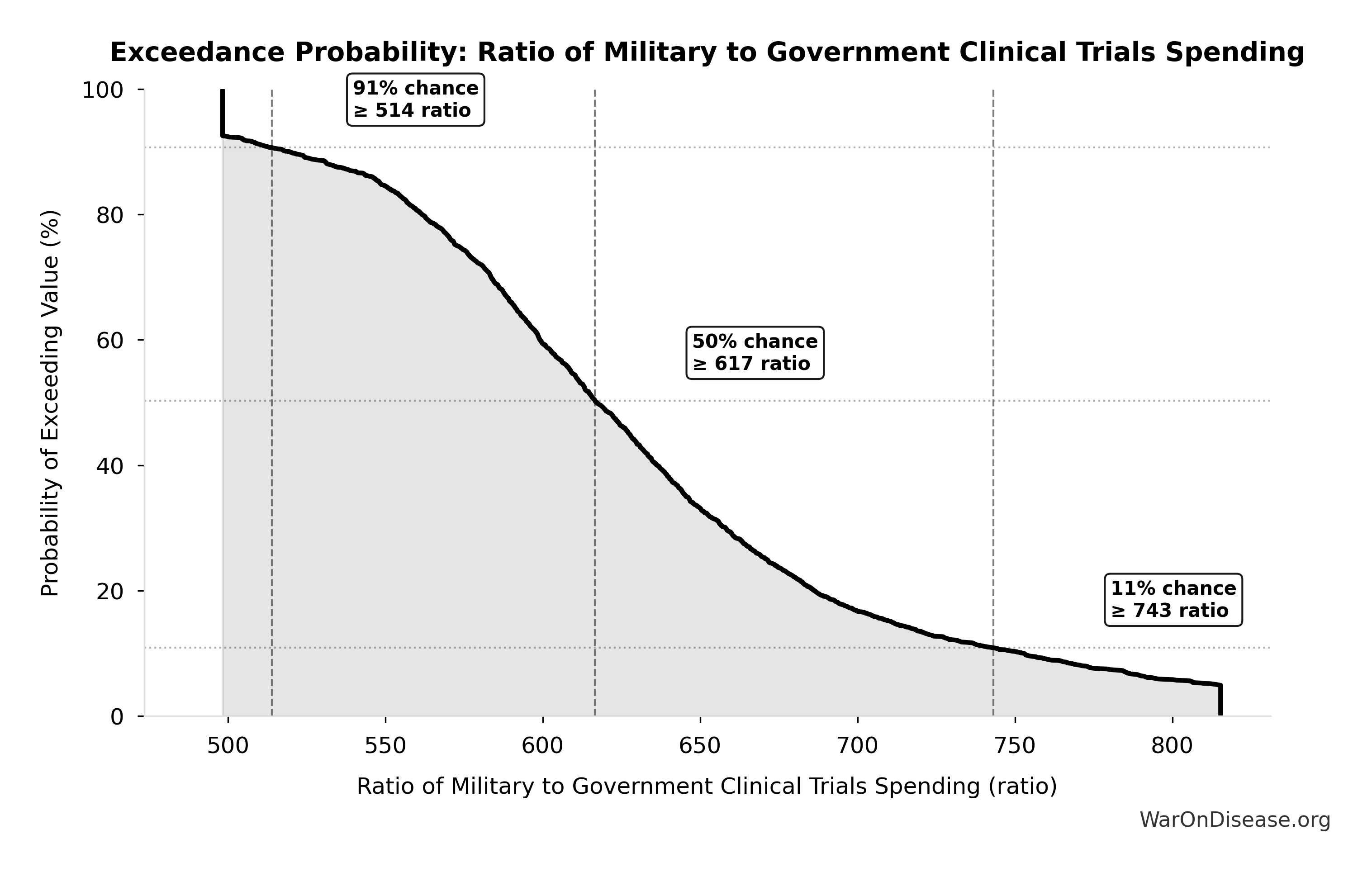
Sensitivity Indices for Annual Cost of Terror Deaths
Regression-based sensitivity showing which inputs explain the most variance in the output.
| Input Parameter | Sensitivity Coefficient | Interpretation |
|---|---|---|
| Value of Statistical Life (USD) | 0.8410 | Strong driver |
| Annual Deaths from Terror Attacks Globally (deaths/year) | 0.5319 | Strong driver |
Interpretation: Standardized coefficients show the change in output (in SD units) per 1 SD change in input. Values near ±1 indicate strong influence; values exceeding ±1 may occur with correlated inputs.
Monte Carlo Distribution
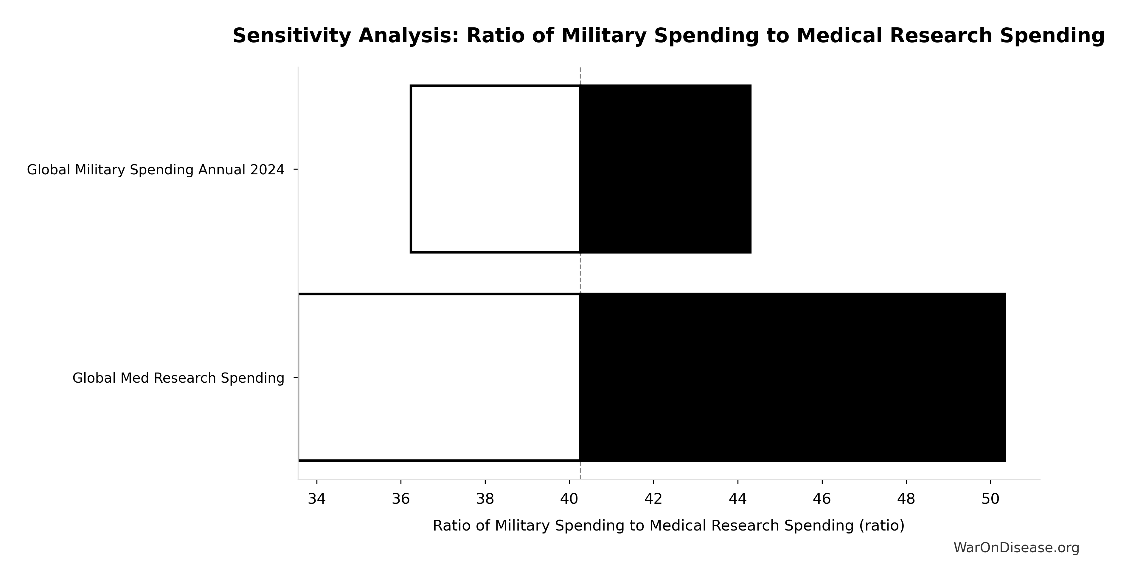
Simulation Results Summary: Annual Cost of Terror Deaths
| Statistic | Value |
|---|---|
| Baseline (deterministic) | $83B |
| Mean (expected value) | $82.1B |
| Median (50th percentile) | $78.9B |
| Standard Deviation | $27B |
| 90% Range (5th-95th percentile) | [$43.1B, $131B] |
The histogram shows the distribution of Annual Cost of Terror Deaths across 10,000 Monte Carlo simulations. The CDF (right) shows the probability of the outcome exceeding any given value, which is useful for risk assessment.
Exceedance Probability
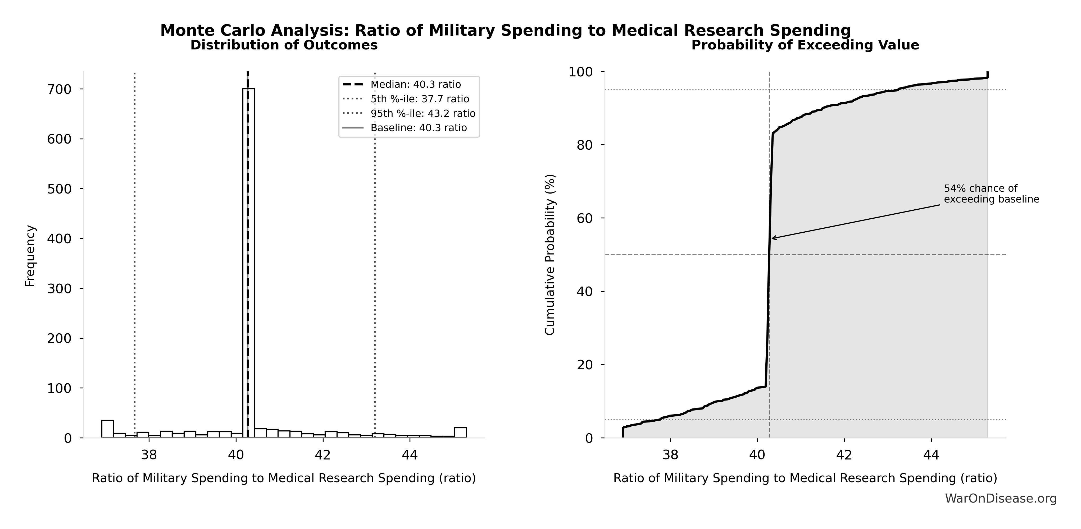
This exceedance probability chart shows the likelihood that Annual Cost of Terror Deaths will exceed any given threshold. Higher curves indicate more favorable outcomes with greater certainty.
Total Annual Human Life Losses from Conflict: $2.45T
Note📊 Details
Total annual human life losses from conflict (sum of combat, terror, state violence)
Inputs:
- Annual Cost of Combat Deaths 🔢: $2.34T
- Annual Cost of State Violence Deaths 🔢: $27B
- Annual Cost of Terror Deaths 🔢: $83B
\[ \begin{gathered} Loss_{life,conflict} \\ = Cost_{combat,human} + Cost_{state,human} \\ + Cost_{terror,human} \\ = \$2.34T + \$27B + \$83B \\ = \$2.45T \end{gathered} \] where: \[ \begin{gathered} Cost_{combat,human} \\ = Deaths_{combat} \times VSL \\ = 234{,}000 \times \$10M \\ = \$2.34T \end{gathered} \] where: \[ \begin{gathered} Cost_{state,human} \\ = Deaths_{state} \times VSL \\ = 2{,}700 \times \$10M \\ = \$27B \end{gathered} \] where: \[ \begin{gathered} Cost_{terror,human} \\ = Deaths_{terror} \times VSL \\ = 8{,}300 \times \$10M \\ = \$83B \end{gathered} \] ✓ High confidence
Sensitivity Analysis
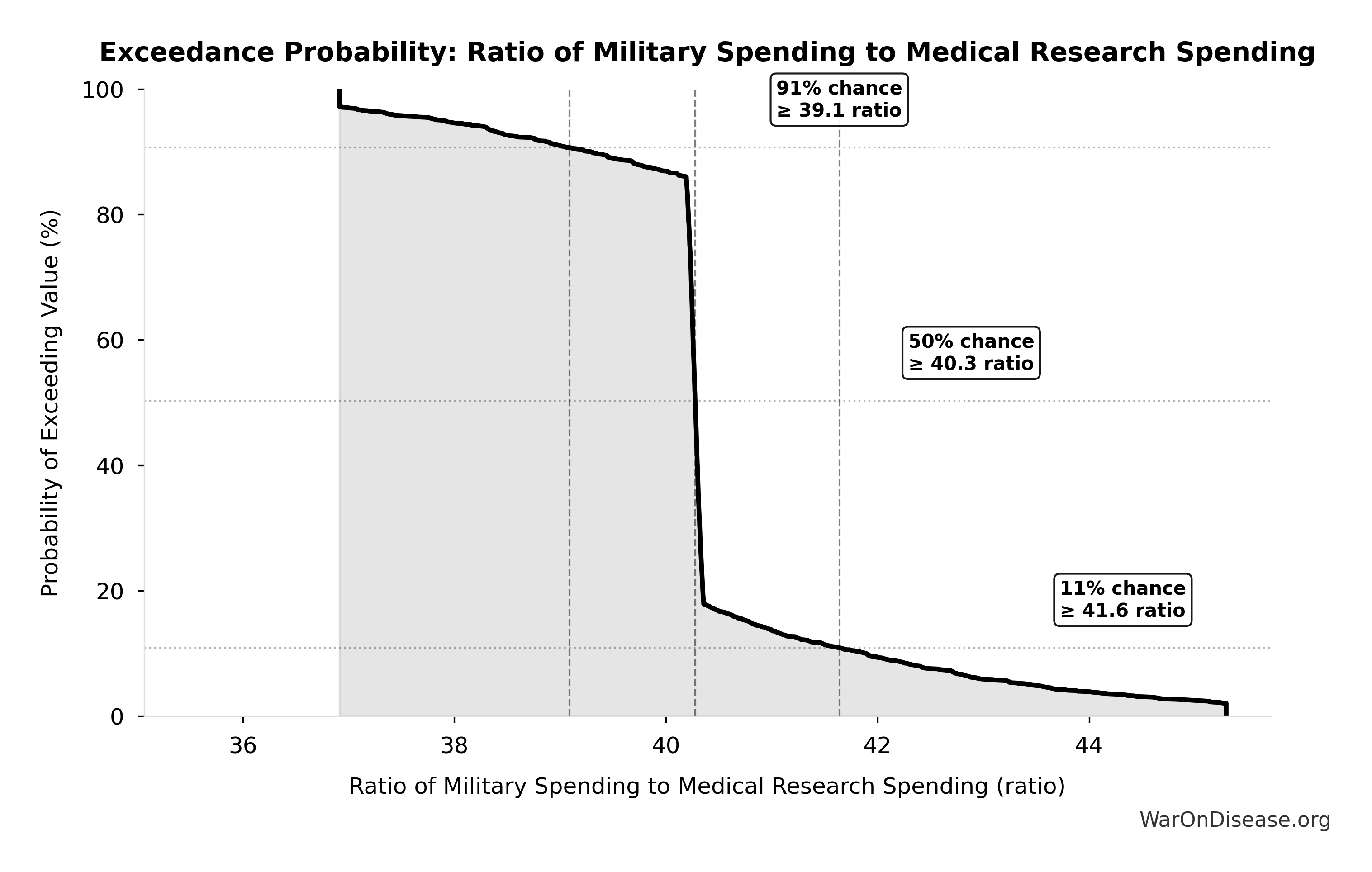
Sensitivity Indices for Total Annual Human Life Losses from Conflict
Regression-based sensitivity showing which inputs explain the most variance in the output.
| Input Parameter | Sensitivity Coefficient | Interpretation |
|---|---|---|
| Annual Cost of Combat Deaths (USD/year) | 0.9500 | Strong driver |
| Annual Cost of Terror Deaths (USD/year) | 0.0365 | Minimal effect |
| Annual Cost of State Violence Deaths (USD/year) | 0.0152 | Minimal effect |
Interpretation: Standardized coefficients show the change in output (in SD units) per 1 SD change in input. Values near ±1 indicate strong influence; values exceeding ±1 may occur with correlated inputs.
Monte Carlo Distribution
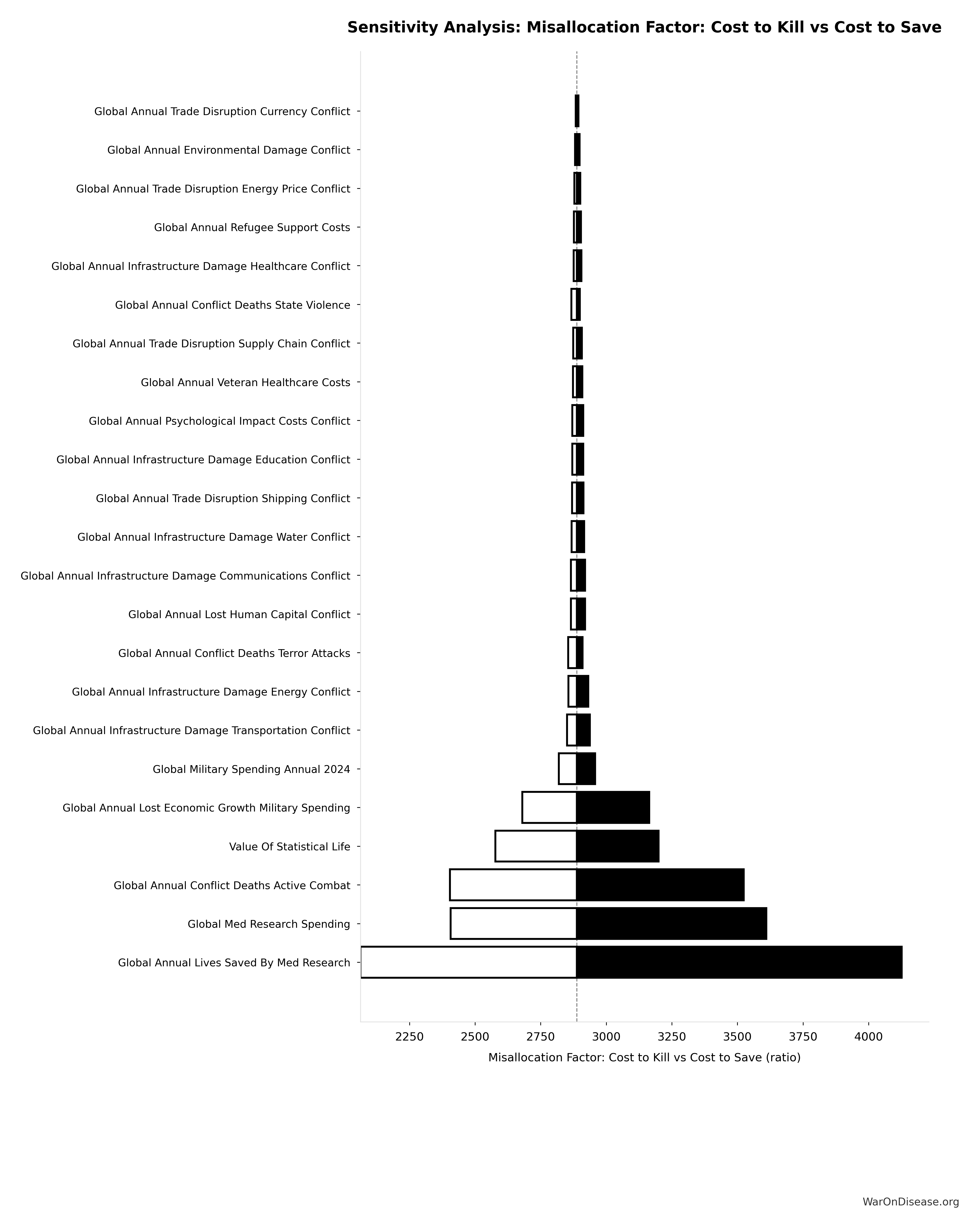
Simulation Results Summary: Total Annual Human Life Losses from Conflict
| Statistic | Value |
|---|---|
| Baseline (deterministic) | $2.45T |
| Mean (expected value) | $2.42T |
| Median (50th percentile) | $2.35T |
| Standard Deviation | $740B |
| 90% Range (5th-95th percentile) | [$1.31T, $3.75T] |
The histogram shows the distribution of Total Annual Human Life Losses from Conflict across 10,000 Monte Carlo simulations. The CDF (right) shows the probability of the outcome exceeding any given value, which is useful for risk assessment.
Exceedance Probability
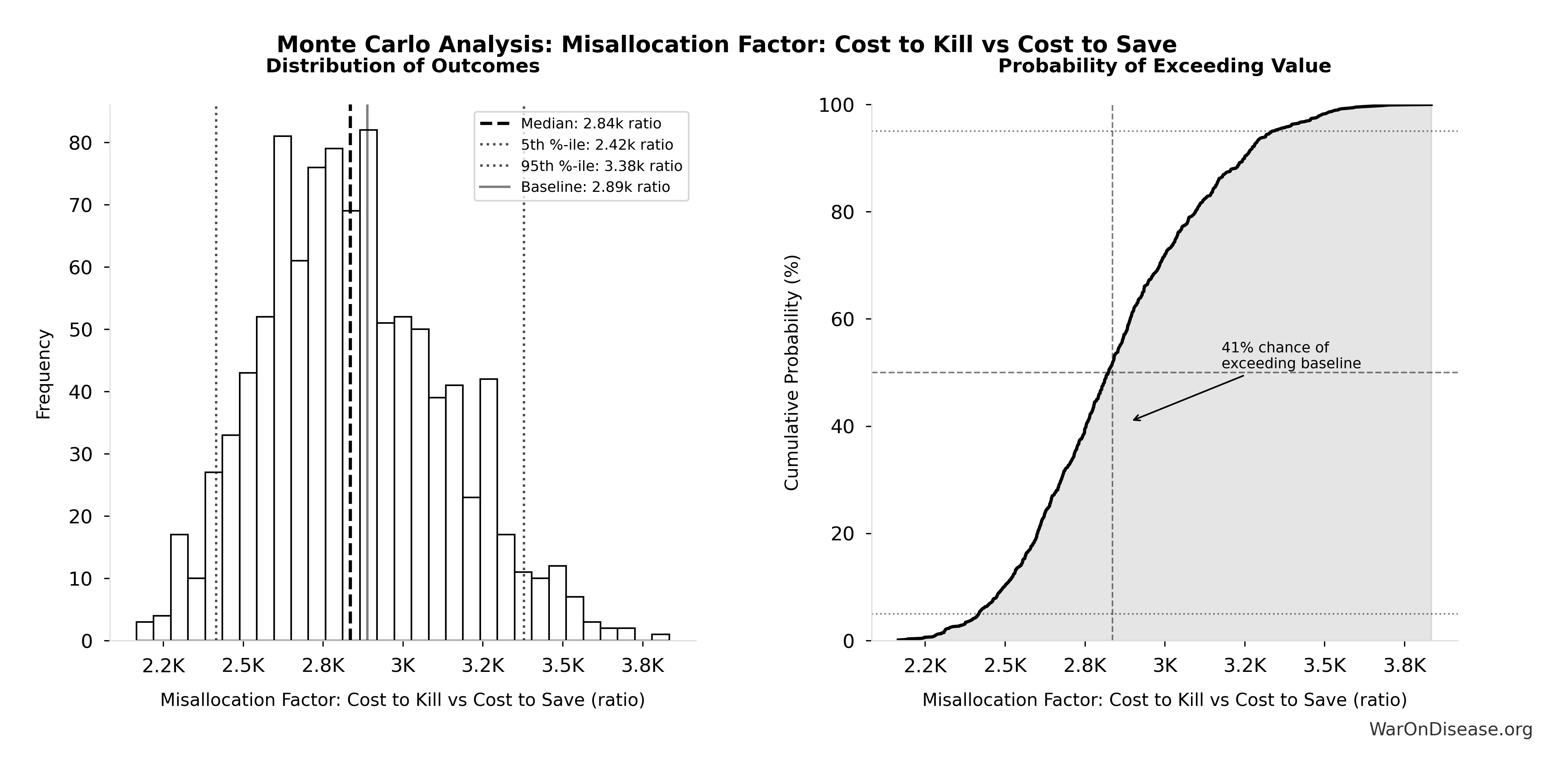
This exceedance probability chart shows the likelihood that Total Annual Human Life Losses from Conflict will exceed any given threshold. Higher curves indicate more favorable outcomes with greater certainty.
Total Annual Infrastructure Destruction: $1.88T
Note📊 Details
Total annual infrastructure destruction (sum of transportation, energy, communications, water, education, healthcare)
Inputs:
- Annual Infrastructure Damage to Communications from Conflict 📊: $298B (95% CI: $209B - $418B)
- Annual Infrastructure Damage to Education Facilities from Conflict 📊: $234B (95% CI: $164B - $328B)
- Annual Infrastructure Damage to Energy Systems from Conflict 📊: $422B (95% CI: $295B - $590B)
- Annual Infrastructure Damage to Healthcare Facilities from Conflict 📊: $166B (95% CI: $116B - $232B)
- Annual Infrastructure Damage to Transportation from Conflict 📊: $487B (95% CI: $340B - $680B)
- Annual Infrastructure Damage to Water Systems from Conflict 📊: $268B (95% CI: $187B - $375B)
\[ \begin{gathered} Damage_{infra,total} \\ = Damage_{comms} + Damage_{edu} + Damage_{energy} \\ + Damage_{health} + Damage_{transport} + Damage_{water} \\ = \$298B + \$234B + \$422B + \$166B + \$487B + \$268B \\ = \$1.88T \end{gathered} \]
✓ High confidence
Sensitivity Analysis
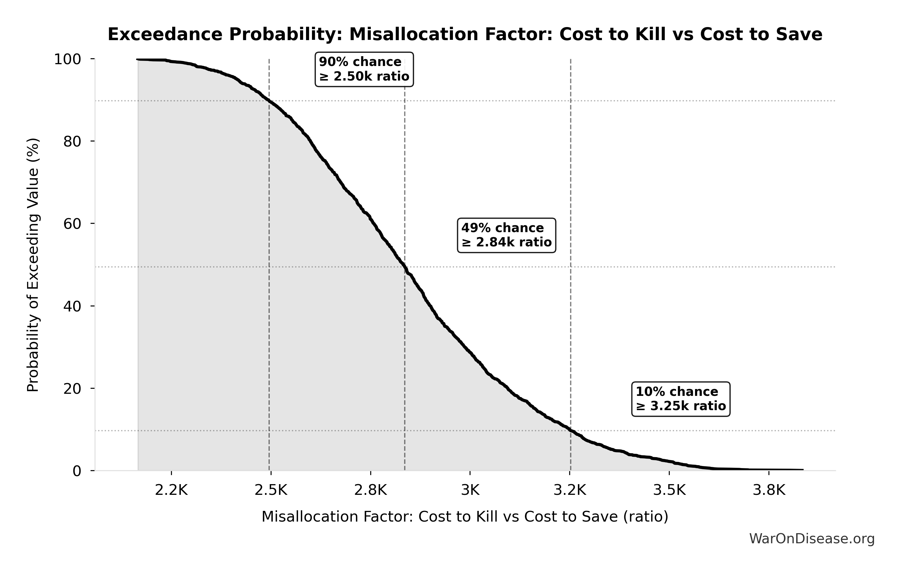
Sensitivity Indices for Total Annual Infrastructure Destruction
Regression-based sensitivity showing which inputs explain the most variance in the output.
| Input Parameter | Sensitivity Coefficient | Interpretation |
|---|---|---|
| Annual Infrastructure Damage to Transportation from Conflict (USD) | 0.2591 | Weak driver |
| Annual Infrastructure Damage to Energy Systems from Conflict (USD) | 0.2249 | Weak driver |
| Annual Infrastructure Damage to Communications from Conflict (USD) | 0.1593 | Weak driver |
| Annual Infrastructure Damage to Water Systems from Conflict (USD) | 0.1433 | Weak driver |
| Annual Infrastructure Damage to Education Facilities from Conflict (USD) | 0.1250 | Weak driver |
| Annual Infrastructure Damage to Healthcare Facilities from Conflict (USD) | 0.0884 | Minimal effect |
Interpretation: Standardized coefficients show the change in output (in SD units) per 1 SD change in input. Values near ±1 indicate strong influence; values exceeding ±1 may occur with correlated inputs.
Monte Carlo Distribution
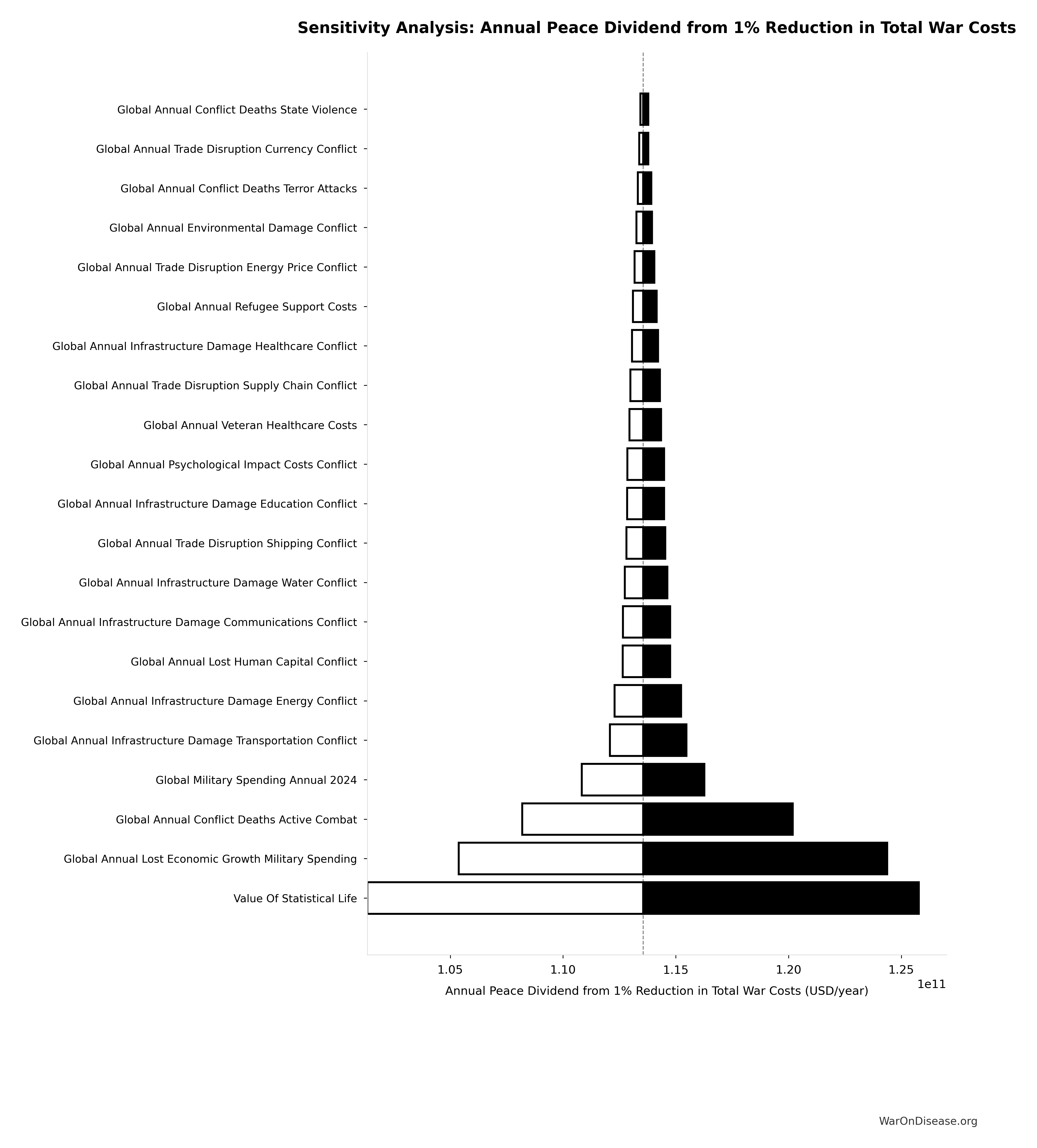
Simulation Results Summary: Total Annual Infrastructure Destruction
| Statistic | Value |
|---|---|
| Baseline (deterministic) | $1.88T |
| Mean (expected value) | $1.87T |
| Median (50th percentile) | $1.84T |
| Standard Deviation | $319B |
| 90% Range (5th-95th percentile) | [$1.37T, $2.47T] |
The histogram shows the distribution of Total Annual Infrastructure Destruction across 10,000 Monte Carlo simulations. The CDF (right) shows the probability of the outcome exceeding any given value, which is useful for risk assessment.
Exceedance Probability
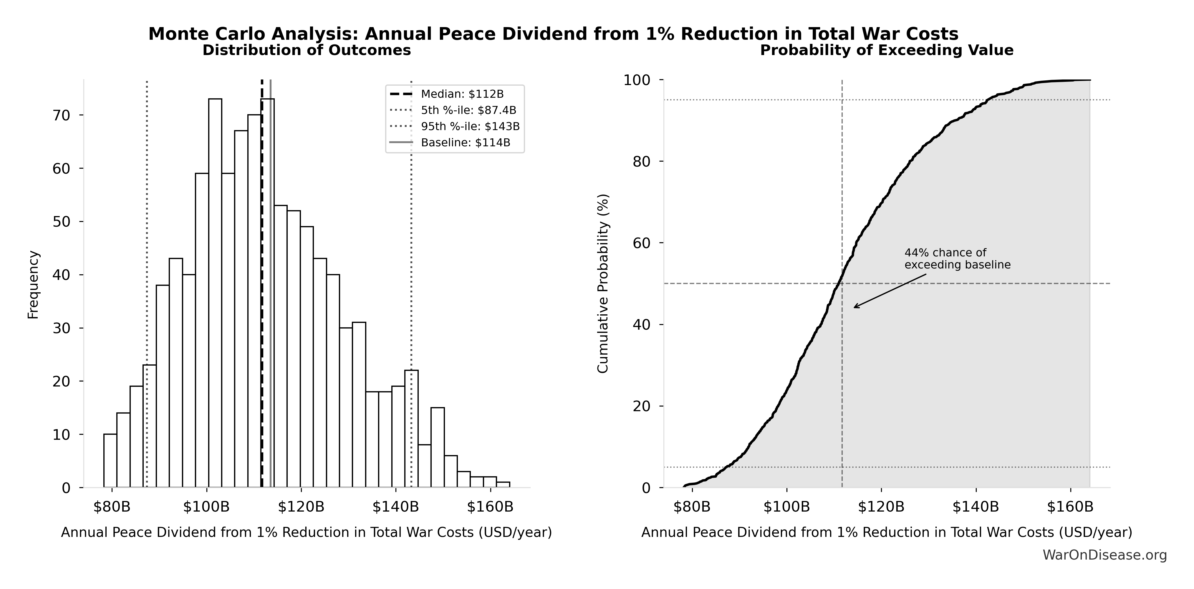
This exceedance probability chart shows the likelihood that Total Annual Infrastructure Destruction will exceed any given threshold. Higher curves indicate more favorable outcomes with greater certainty.
Total Annual Trade Disruption: $616B
Note📊 Details
Total annual trade disruption (sum of shipping, supply chain, energy prices, currency instability)
Inputs:
- Annual Trade Disruption Costs from Currency Instability 📊: $57.4B (95% CI: $40B - $80B)
- Annual Trade Disruption Costs from Energy Price Volatility 📊: $125B (95% CI: $87B - $175B)
- Annual Trade Disruption Costs from Shipping Disruptions 📊: $247B (95% CI: $173B - $346B)
- Annual Trade Disruption Costs from Supply Chain Disruptions 📊: $187B (95% CI: $131B - $262B)
\[ \begin{gathered} Disruption_{trade} \\ = Disruption_{currency} + Disruption_{energy} \\ + Disruption_{shipping} + Disruption_{supply} \\ = \$57.4B + \$125B + \$247B + \$187B \\ = \$616B \end{gathered} \]
✓ High confidence
Sensitivity Analysis
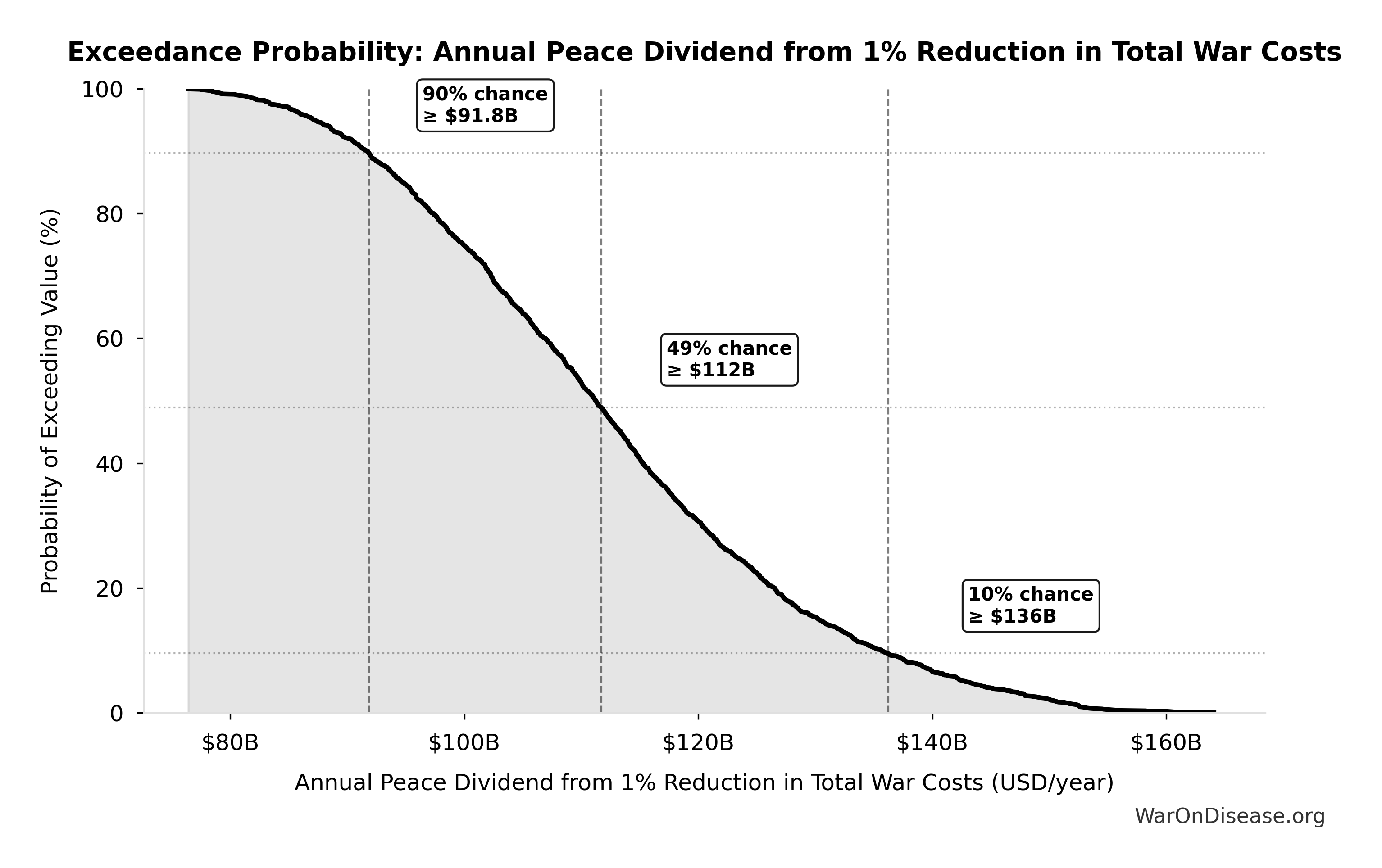
Sensitivity Indices for Total Annual Trade Disruption
Regression-based sensitivity showing which inputs explain the most variance in the output.
| Input Parameter | Sensitivity Coefficient | Interpretation |
|---|---|---|
| Annual Trade Disruption Costs from Shipping Disruptions (USD) | 0.4005 | Moderate driver |
| Annual Trade Disruption Costs from Supply Chain Disruptions (USD) | 0.3033 | Moderate driver |
| Annual Trade Disruption Costs from Energy Price Volatility (USD) | 0.2037 | Weak driver |
| Annual Trade Disruption Costs from Currency Instability (USD) | 0.0926 | Minimal effect |
Interpretation: Standardized coefficients show the change in output (in SD units) per 1 SD change in input. Values near ±1 indicate strong influence; values exceeding ±1 may occur with correlated inputs.
Monte Carlo Distribution
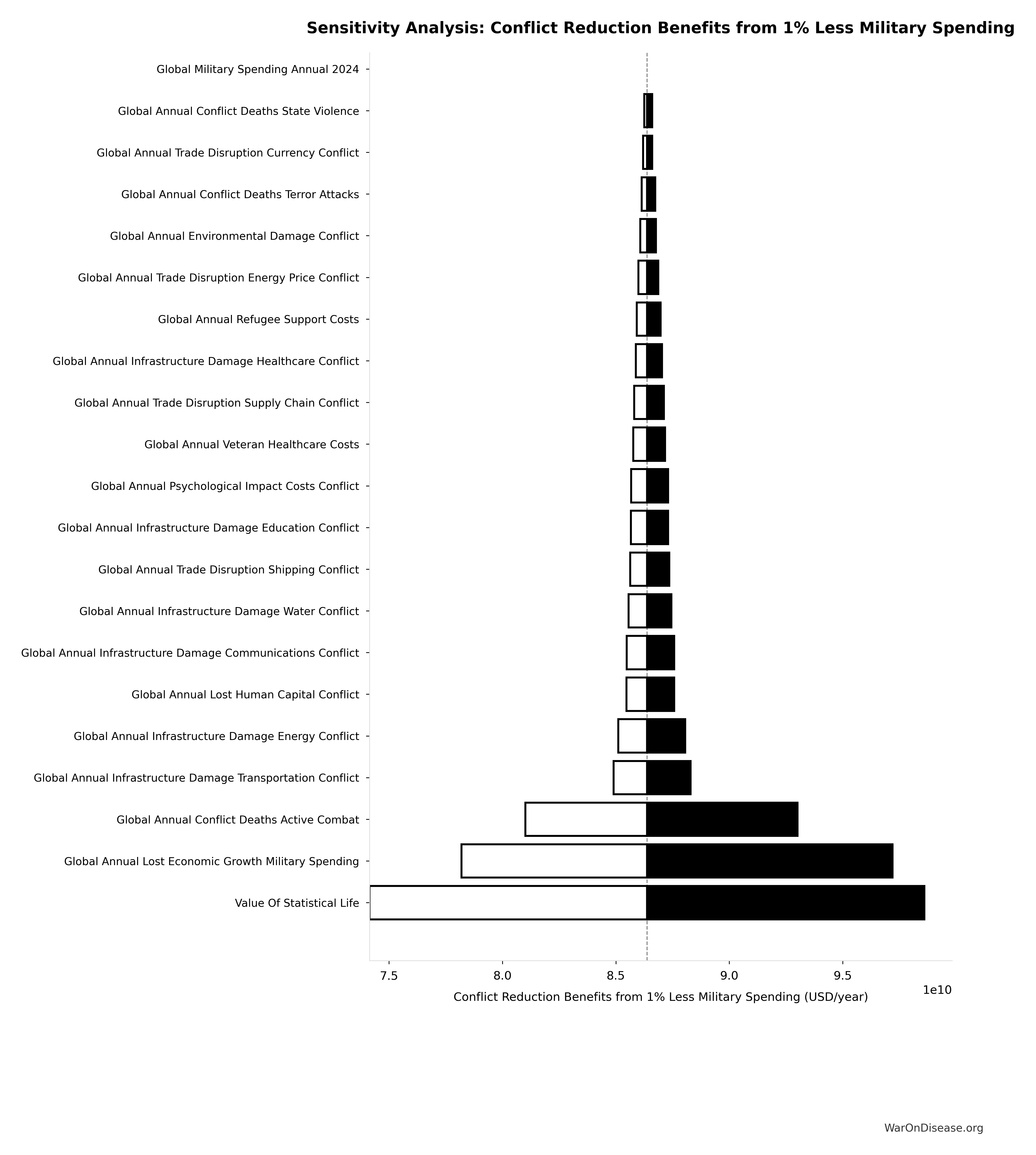
Simulation Results Summary: Total Annual Trade Disruption
| Statistic | Value |
|---|---|
| Baseline (deterministic) | $616B |
| Mean (expected value) | $614B |
| Median (50th percentile) | $605B |
| Standard Deviation | $105B |
| 90% Range (5th-95th percentile) | [$450B, $812B] |
The histogram shows the distribution of Total Annual Trade Disruption across 10,000 Monte Carlo simulations. The CDF (right) shows the probability of the outcome exceeding any given value, which is useful for risk assessment.
Exceedance Probability
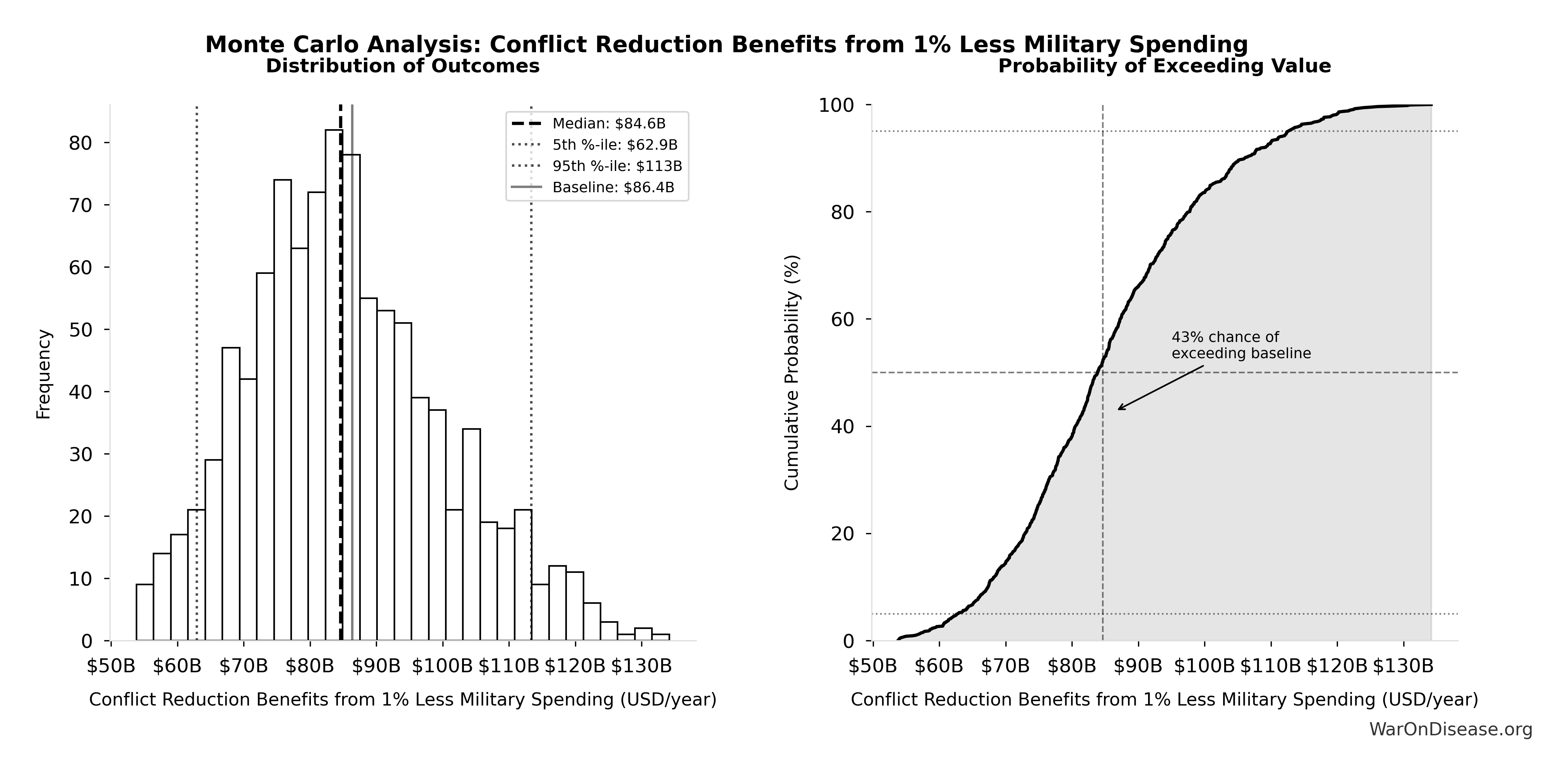
This exceedance probability chart shows the likelihood that Total Annual Trade Disruption will exceed any given threshold. Higher curves indicate more favorable outcomes with greater certainty.
Total Annual Direct War Costs: $7.66T
Note📊 Details
Total annual direct war costs (military spending + infrastructure + human life + trade disruption)
Inputs:
- Total Annual Human Life Losses from Conflict 🔢: $2.45T
- Total Annual Infrastructure Destruction 🔢: $1.88T
- Total Annual Trade Disruption 🔢: $616B
- Global Military Spending in 2024 📊: $2.72T
\[ \begin{gathered} Cost_{war,direct} \\ = Loss_{life,conflict} + Damage_{infra,total} \\ + Disruption_{trade} + Spending_{mil} \\ = \$2.45T + \$1.88T + \$616B + \$2.72T \\ = \$7.66T \end{gathered} \] where: \[ \begin{gathered} Loss_{life,conflict} \\ = Cost_{combat,human} + Cost_{state,human} \\ + Cost_{terror,human} \\ = \$2.34T + \$27B + \$83B \\ = \$2.45T \end{gathered} \] where: \[ \begin{gathered} Cost_{combat,human} \\ = Deaths_{combat} \times VSL \\ = 234{,}000 \times \$10M \\ = \$2.34T \end{gathered} \] where: \[ \begin{gathered} Cost_{state,human} \\ = Deaths_{state} \times VSL \\ = 2{,}700 \times \$10M \\ = \$27B \end{gathered} \] where: \[ \begin{gathered} Cost_{terror,human} \\ = Deaths_{terror} \times VSL \\ = 8{,}300 \times \$10M \\ = \$83B \end{gathered} \] where: \[ \begin{gathered} Damage_{infra,total} \\ = Damage_{comms} + Damage_{edu} + Damage_{energy} \\ + Damage_{health} + Damage_{transport} + Damage_{water} \\ = \$298B + \$234B + \$422B + \$166B + \$487B + \$268B \\ = \$1.88T \end{gathered} \] where: \[ \begin{gathered} Disruption_{trade} \\ = Disruption_{currency} + Disruption_{energy} \\ + Disruption_{shipping} + Disruption_{supply} \\ = \$57.4B + \$125B + \$247B + \$187B \\ = \$616B \end{gathered} \] ✓ High confidence
Sensitivity Analysis
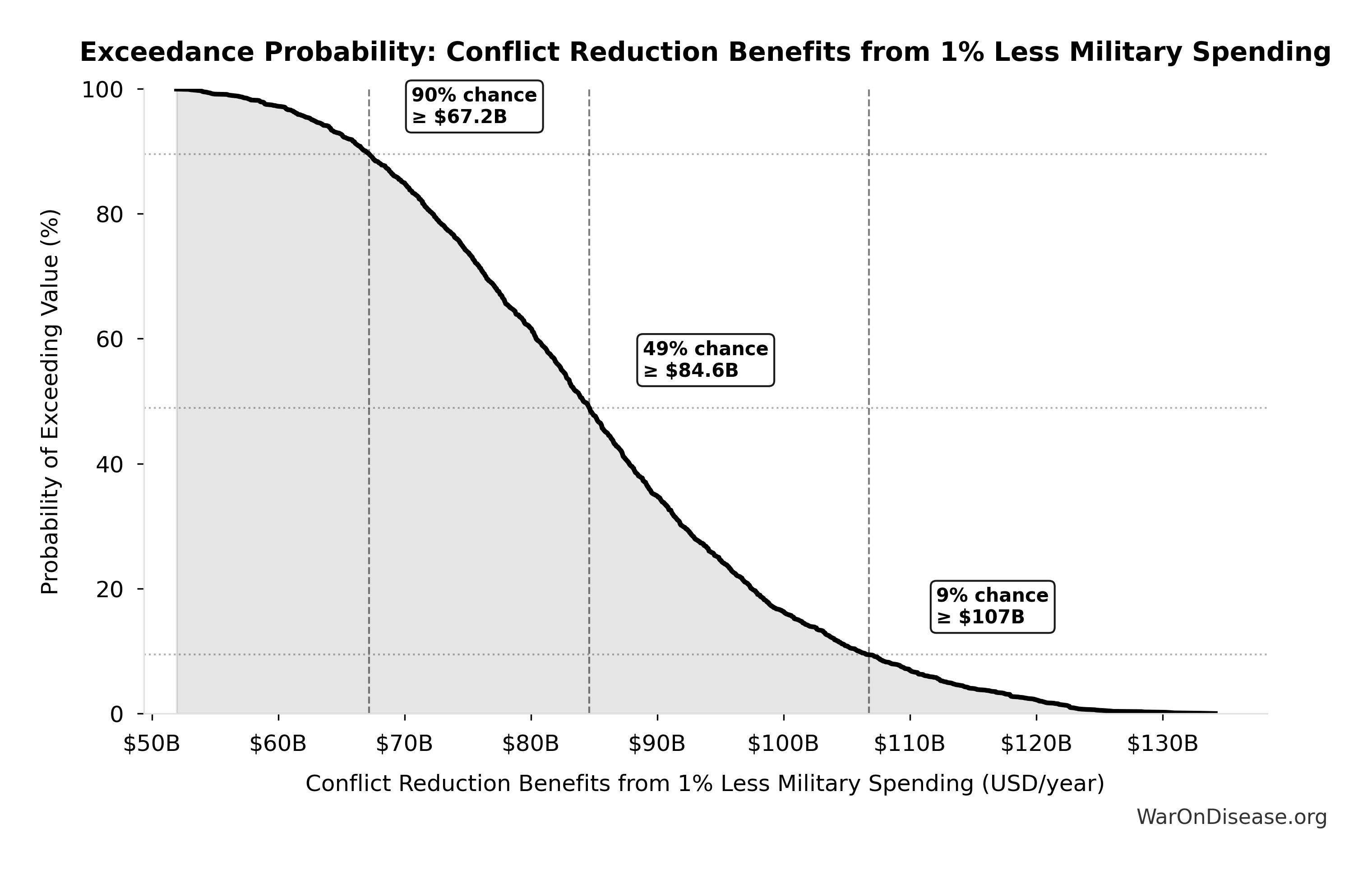
Sensitivity Indices for Total Annual Direct War Costs
Regression-based sensitivity showing which inputs explain the most variance in the output.
| Input Parameter | Sensitivity Coefficient | Interpretation |
|---|---|---|
| Total Annual Human Life Losses from Conflict (USD/year) | 0.7463 | Strong driver |
| Total Annual Infrastructure Destruction (USD/year) | 0.3211 | Moderate driver |
| Total Annual Trade Disruption (USD/year) | 0.1057 | Weak driver |
Interpretation: Standardized coefficients show the change in output (in SD units) per 1 SD change in input. Values near ±1 indicate strong influence; values exceeding ±1 may occur with correlated inputs.
Monte Carlo Distribution
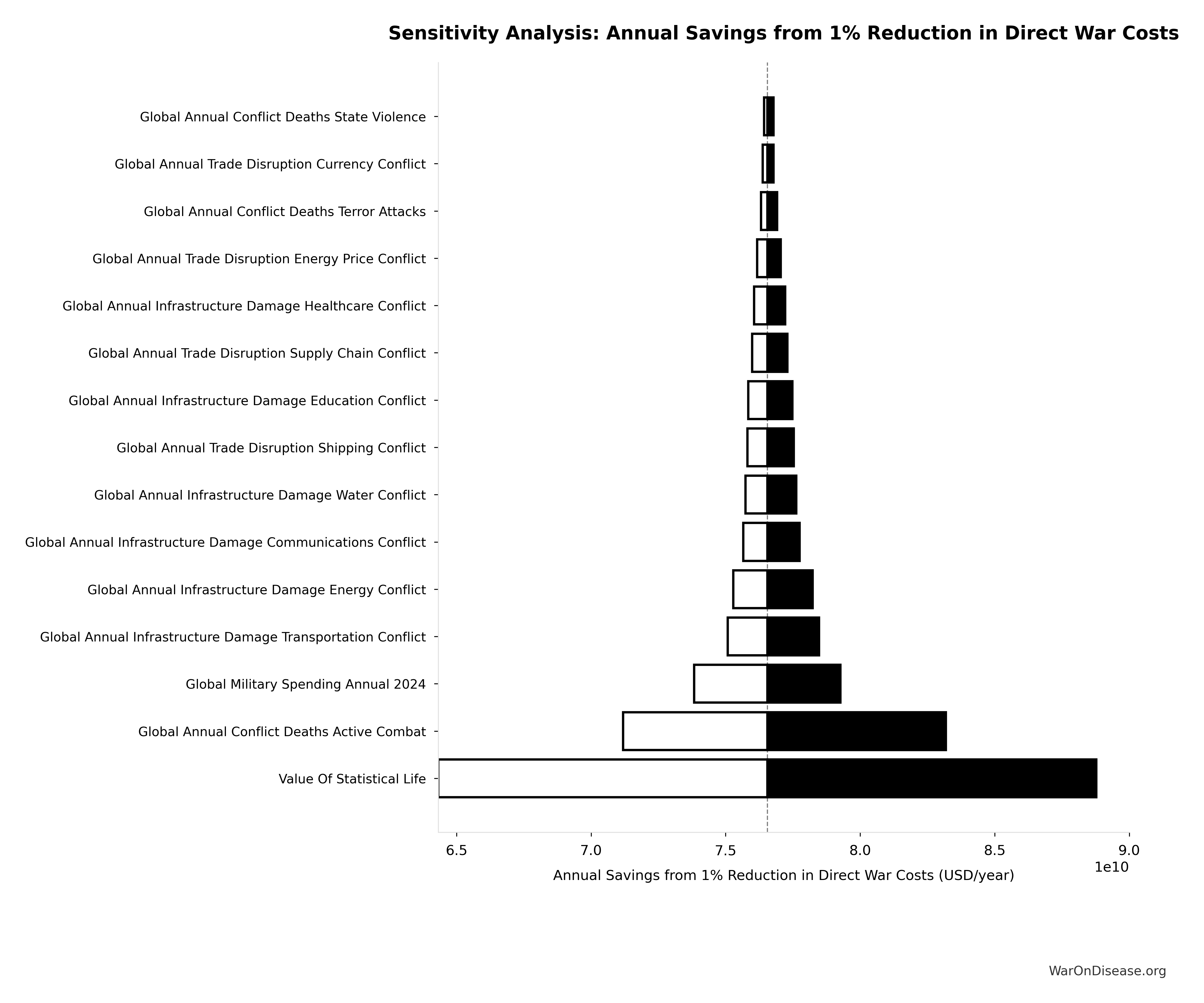
Simulation Results Summary: Total Annual Direct War Costs
| Statistic | Value |
|---|---|
| Baseline (deterministic) | $7.66T |
| Mean (expected value) | $7.62T |
| Median (50th percentile) | $7.53T |
| Standard Deviation | $992B |
| 90% Range (5th-95th percentile) | [$6.14T, $9.4T] |
The histogram shows the distribution of Total Annual Direct War Costs across 10,000 Monte Carlo simulations. The CDF (right) shows the probability of the outcome exceeding any given value, which is useful for risk assessment.
Exceedance Probability
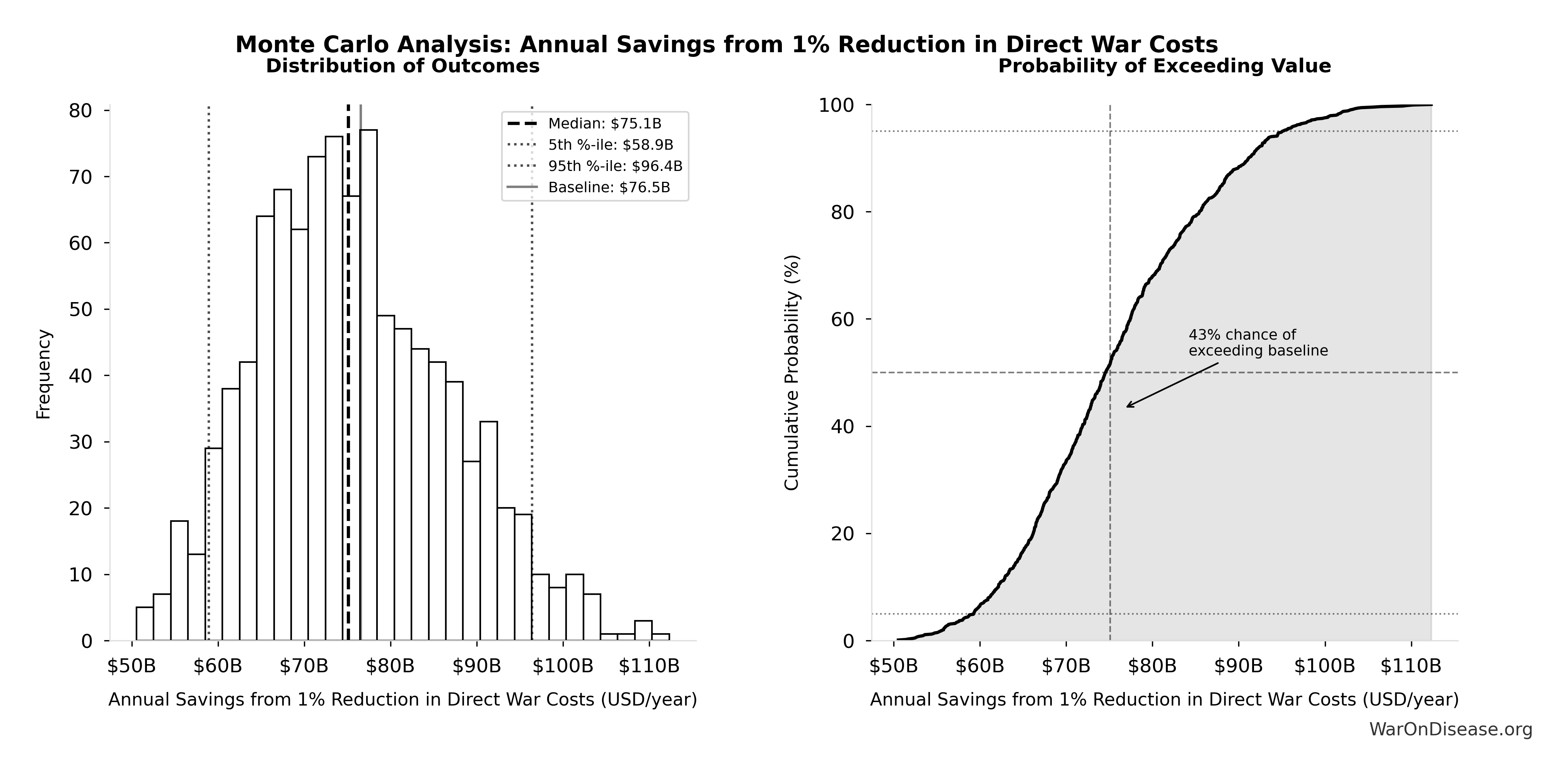
This exceedance probability chart shows the likelihood that Total Annual Direct War Costs will exceed any given threshold. Higher curves indicate more favorable outcomes with greater certainty.
Total Annual Indirect War Costs: $3.7T
Note📊 Details
Total annual indirect war costs (opportunity cost + veterans + refugees + environment + mental health + lost productivity)
Inputs:
- Annual Environmental Damage and Restoration Costs from Conflict 📊: $100B (95% CI: $70B - $140B)
- Annual Lost Economic Growth from Military Spending Opportunity Cost 📊: $2.72T (95% CI: $1.9T - $3.8T)
- Annual Lost Productivity from Conflict Casualties 📊: $300B (95% CI: $210B - $420B)
- Annual PTSD and Mental Health Costs from Conflict 📊: $232B (95% CI: $162B - $325B)
- Annual Refugee Support Costs 📊: $150B (95% CI: $105B - $210B)
- Annual Veteran Healthcare Costs 📊: $200B (95% CI: $140B - $280B)
\[ \begin{gathered} Cost_{war,indirect} \\ = Damage_{env} + Loss_{growth,mil} + Loss_{capital,conflict} \\ + Cost_{psych} + Cost_{refugee} + Cost_{vet} \\ = \$100B + \$2.72T + \$300B + \$232B + \$150B + \$200B \\ = \$3.7T \end{gathered} \]
✓ High confidence
Sensitivity Analysis
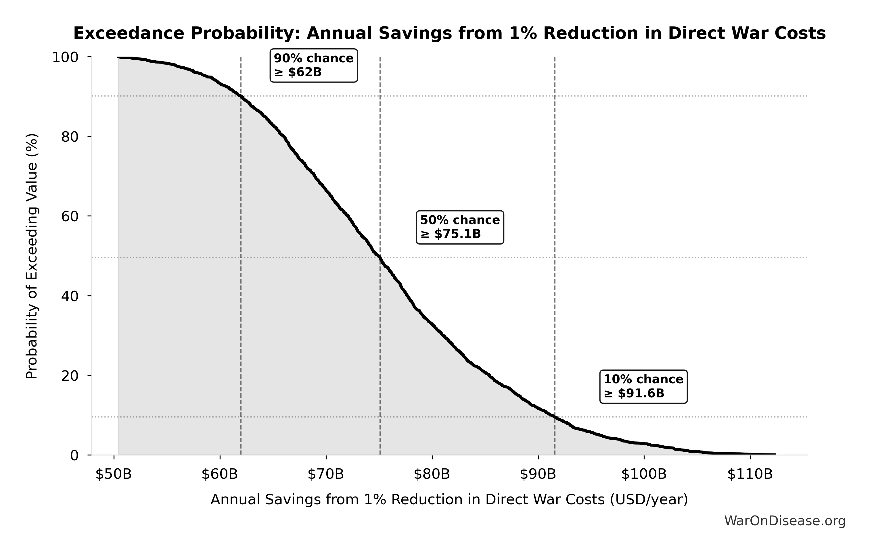
Sensitivity Indices for Total Annual Indirect War Costs
Regression-based sensitivity showing which inputs explain the most variance in the output.
| Input Parameter | Sensitivity Coefficient | Interpretation |
|---|---|---|
| Annual Refugee Support Costs (USD) | 3.5996 | Strong driver |
| Annual Lost Productivity from Conflict Casualties (USD) | -1.9754 | Strong driver |
| Annual Environmental Damage and Restoration Costs from Conflict (USD) | -1.4754 | Strong driver |
| Annual Lost Economic Growth from Military Spending Opportunity Cost (USD) | 0.7342 | Strong driver |
| Annual PTSD and Mental Health Costs from Conflict (USD) | 0.0630 | Minimal effect |
| Annual Veteran Healthcare Costs (USD) | 0.0541 | Minimal effect |
Interpretation: Standardized coefficients show the change in output (in SD units) per 1 SD change in input. Values near ±1 indicate strong influence; values exceeding ±1 may occur with correlated inputs.
Monte Carlo Distribution
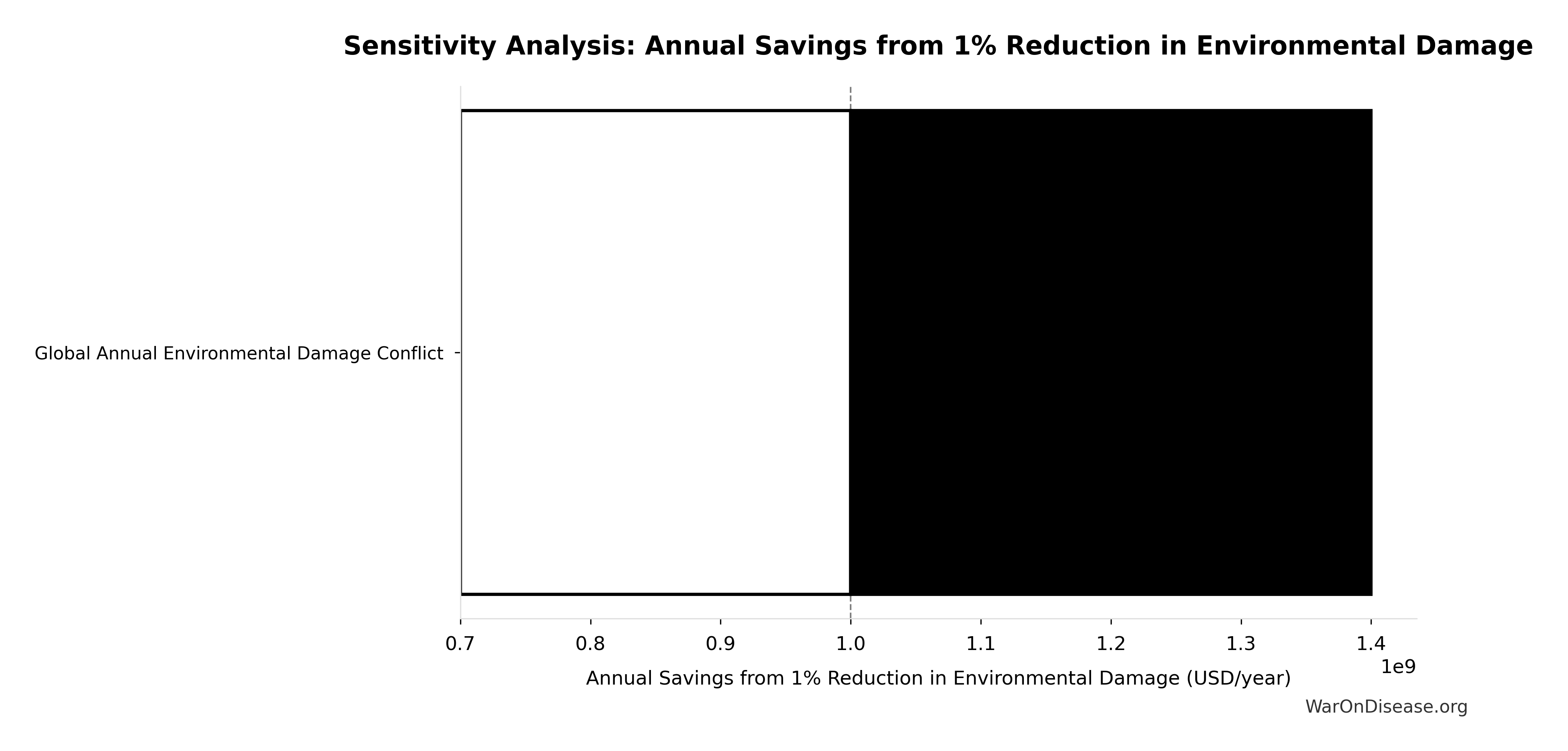
Simulation Results Summary: Total Annual Indirect War Costs
| Statistic | Value |
|---|---|
| Baseline (deterministic) | $3.7T |
| Mean (expected value) | $3.69T |
| Median (50th percentile) | $3.63T |
| Standard Deviation | $628B |
| 90% Range (5th-95th percentile) | [$2.71T, $4.87T] |
The histogram shows the distribution of Total Annual Indirect War Costs across 10,000 Monte Carlo simulations. The CDF (right) shows the probability of the outcome exceeding any given value, which is useful for risk assessment.
Exceedance Probability
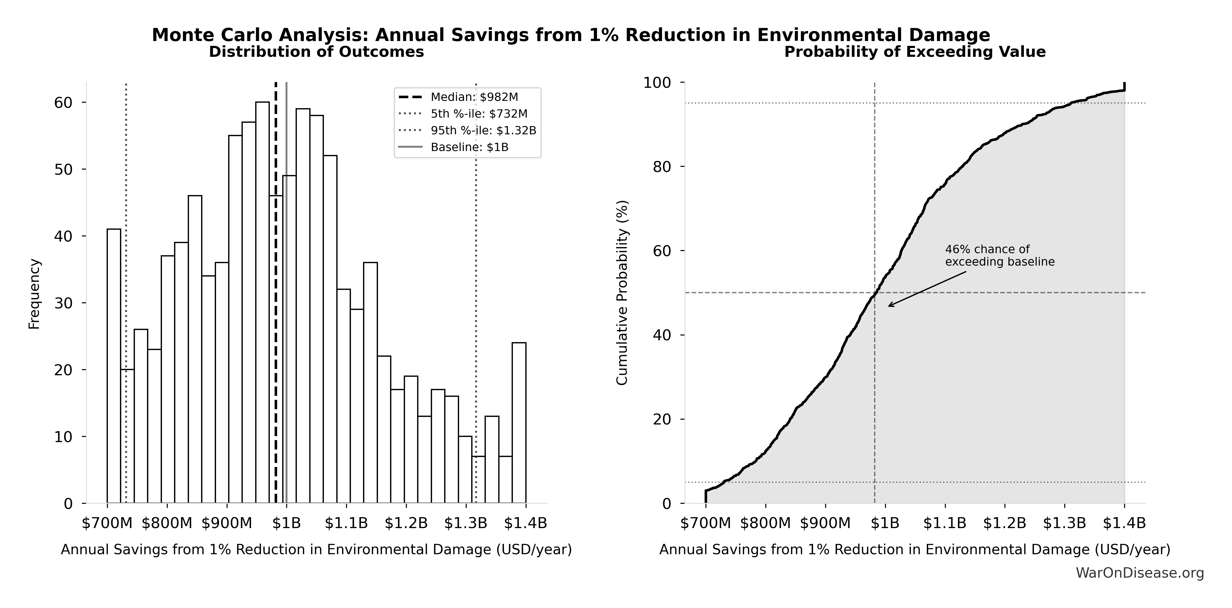
This exceedance probability chart shows the likelihood that Total Annual Indirect War Costs will exceed any given threshold. Higher curves indicate more favorable outcomes with greater certainty.
Annual Welfare Cost of Avoidable Disease: $400T
Note📊 Details
Annual welfare cost of avoidable disease globally. Calculated as global DALY burden × eventually avoidable percentage × standard QALY value ($150K). Uses consistent QALY valuation matching all other health impact calculations. Medical costs and productivity losses are NOT added separately to avoid double-counting (QALY valuation already captures these welfare components).
Inputs:
- Global Annual DALY Burden 📊: 2.88 billion DALYs/year (SE: ±150 million DALYs/year)
- Eventually Avoidable DALY Percentage: 92.6% (95% CI: 50% - 98%)
- Standard Economic Value per QALY 📊: $150K (SE: ±$30K)
\[ \begin{gathered} Burden_{disease} \\ = DALYs_{global,ann} \times Pct_{avoid,DALY} \times Value_{QALY} \\ = 2.88B \times 92.6\% \times \$150K \\ = \$400T \end{gathered} \]
✓ High confidence
Sensitivity Analysis
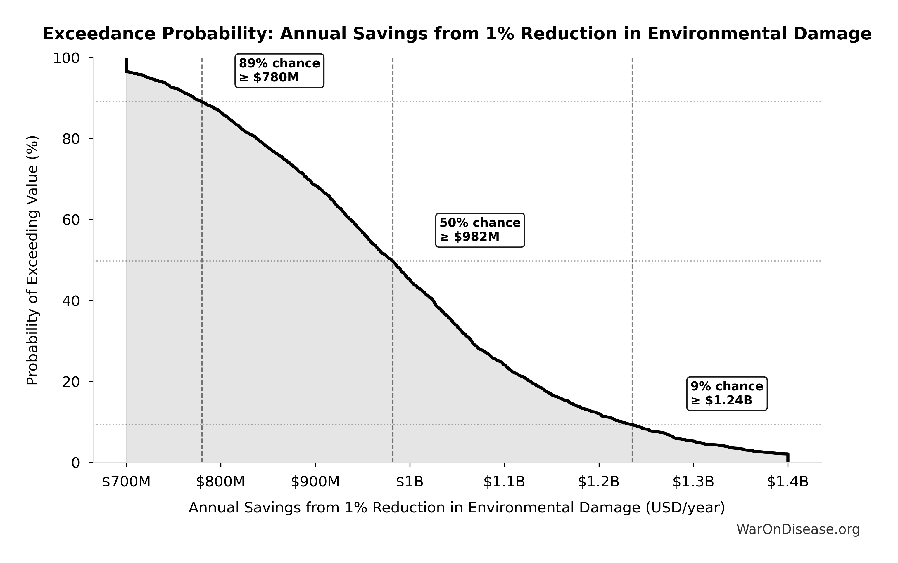
Sensitivity Indices for Annual Welfare Cost of Avoidable Disease
Regression-based sensitivity showing which inputs explain the most variance in the output.
| Input Parameter | Sensitivity Coefficient | Interpretation |
|---|---|---|
| Standard Economic Value per QALY (USD/QALY) | 0.6906 | Strong driver |
| Eventually Avoidable DALY Percentage (percentage) | 0.4534 | Moderate driver |
| Global Annual DALY Burden (DALYs/year) | 0.2031 | Weak driver |
Interpretation: Standardized coefficients show the change in output (in SD units) per 1 SD change in input. Values near ±1 indicate strong influence; values exceeding ±1 may occur with correlated inputs.
Monte Carlo Distribution
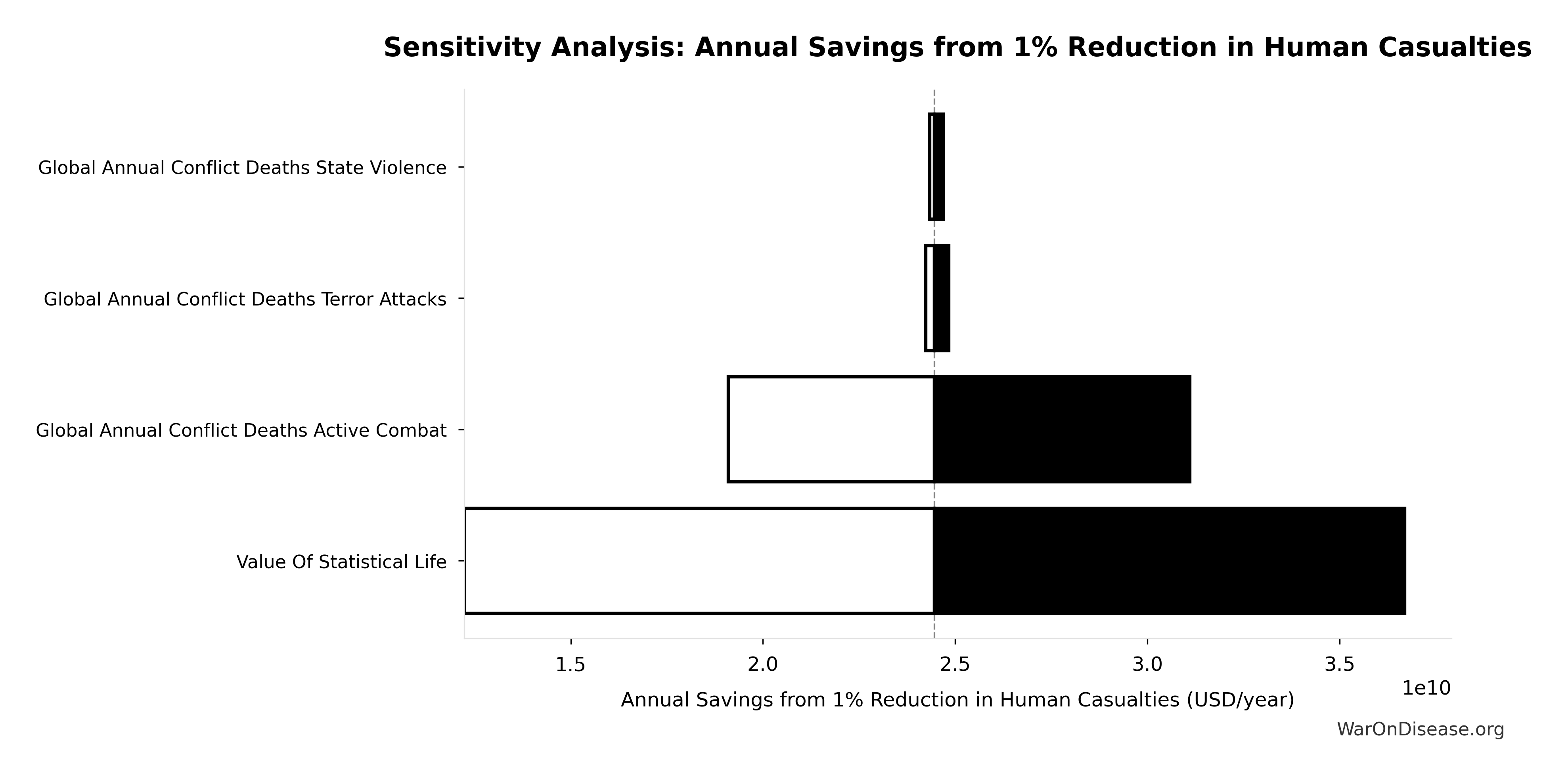
Simulation Results Summary: Annual Welfare Cost of Avoidable Disease
| Statistic | Value |
|---|---|
| Baseline (deterministic) | $400T |
| Mean (expected value) | $400T |
| Median (50th percentile) | $397T |
| Standard Deviation | $105T |
| 90% Range (5th-95th percentile) | [$240T, $587T] |
The histogram shows the distribution of Annual Welfare Cost of Avoidable Disease across 10,000 Monte Carlo simulations. The CDF (right) shows the probability of the outcome exceeding any given value, which is useful for risk assessment.
Exceedance Probability
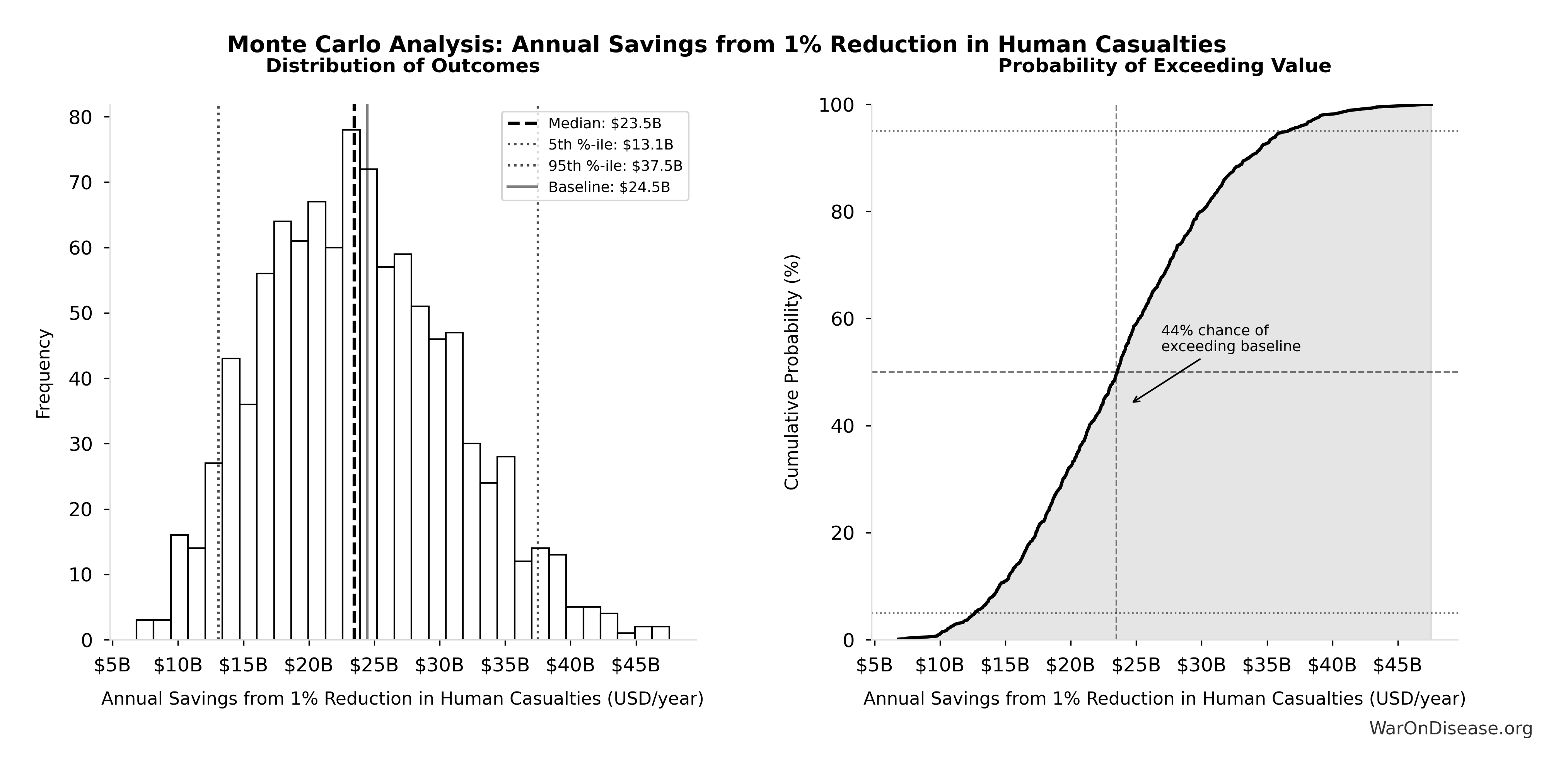
This exceedance probability chart shows the likelihood that Annual Welfare Cost of Avoidable Disease will exceed any given threshold. Higher curves indicate more favorable outcomes with greater certainty.
Total Annual Cost of War and Disease: $412T
Note📊 Details
Total annual welfare cost of war and disease. Disease burden uses DALY-based welfare valuation; war costs use direct + indirect economic costs. Symptomatic treatment costs NOT added separately (already captured in QALY valuation).
Inputs:
- Total Annual Cost of War Worldwide 🔢: $11.4T
- Annual Welfare Cost of Avoidable Disease 🔢: $400T
\[ \begin{gathered} Cost_{health+war} \\ = Cost_{war,total} + Burden_{disease} \\ = \$11.4T + \$400T \\ = \$412T \end{gathered} \] where: \[ \begin{gathered} Cost_{war,total} \\ = Cost_{war,direct} + Cost_{war,indirect} \\ = \$7.66T + \$3.7T \\ = \$11.4T \end{gathered} \] where: \[ \begin{gathered} Cost_{war,direct} \\ = Loss_{life,conflict} + Damage_{infra,total} \\ + Disruption_{trade} + Spending_{mil} \\ = \$2.45T + \$1.88T + \$616B + \$2.72T \\ = \$7.66T \end{gathered} \] where: \[ \begin{gathered} Loss_{life,conflict} \\ = Cost_{combat,human} + Cost_{state,human} \\ + Cost_{terror,human} \\ = \$2.34T + \$27B + \$83B \\ = \$2.45T \end{gathered} \] where: \[ \begin{gathered} Cost_{combat,human} \\ = Deaths_{combat} \times VSL \\ = 234{,}000 \times \$10M \\ = \$2.34T \end{gathered} \] where: \[ \begin{gathered} Cost_{state,human} \\ = Deaths_{state} \times VSL \\ = 2{,}700 \times \$10M \\ = \$27B \end{gathered} \] where: \[ \begin{gathered} Cost_{terror,human} \\ = Deaths_{terror} \times VSL \\ = 8{,}300 \times \$10M \\ = \$83B \end{gathered} \] where: \[ \begin{gathered} Damage_{infra,total} \\ = Damage_{comms} + Damage_{edu} + Damage_{energy} \\ + Damage_{health} + Damage_{transport} + Damage_{water} \\ = \$298B + \$234B + \$422B + \$166B + \$487B + \$268B \\ = \$1.88T \end{gathered} \] where: \[ \begin{gathered} Disruption_{trade} \\ = Disruption_{currency} + Disruption_{energy} \\ + Disruption_{shipping} + Disruption_{supply} \\ = \$57.4B + \$125B + \$247B + \$187B \\ = \$616B \end{gathered} \] where: \[ \begin{gathered} Cost_{war,indirect} \\ = Damage_{env} + Loss_{growth,mil} + Loss_{capital,conflict} \\ + Cost_{psych} + Cost_{refugee} + Cost_{vet} \\ = \$100B + \$2.72T + \$300B + \$232B + \$150B + \$200B \\ = \$3.7T \end{gathered} \] where: \[ \begin{gathered} Burden_{disease} \\ = DALYs_{global,ann} \times Pct_{avoid,DALY} \times Value_{QALY} \\ = 2.88B \times 92.6\% \times \$150K \\ = \$400T \end{gathered} \] ✓ High confidence
Sensitivity Analysis
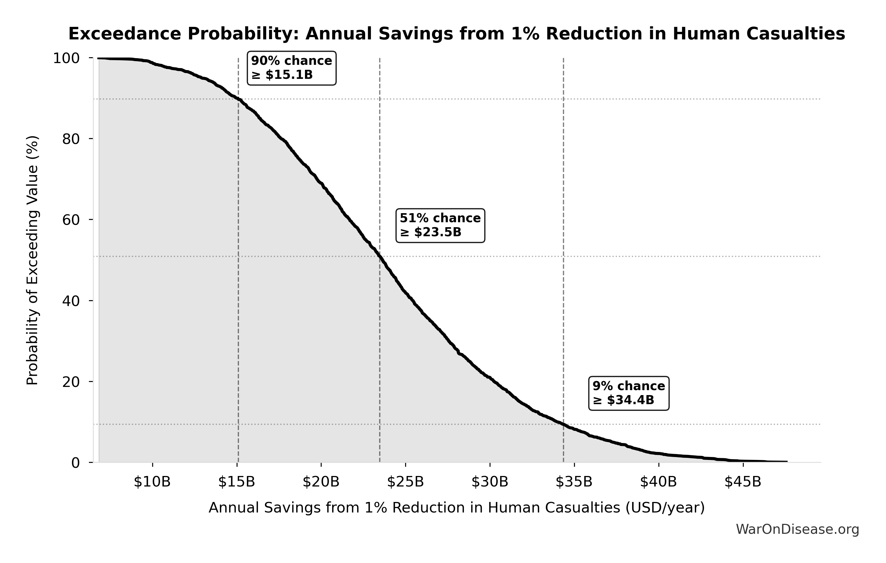
Sensitivity Indices for Total Annual Cost of War and Disease
Regression-based sensitivity showing which inputs explain the most variance in the output.
| Input Parameter | Sensitivity Coefficient | Interpretation |
|---|---|---|
| Annual Welfare Cost of Avoidable Disease (USD/year) | 0.9886 | Strong driver |
| Total Annual Cost of War Worldwide (USD/year) | 0.0143 | Minimal effect |
Interpretation: Standardized coefficients show the change in output (in SD units) per 1 SD change in input. Values near ±1 indicate strong influence; values exceeding ±1 may occur with correlated inputs.
Monte Carlo Distribution
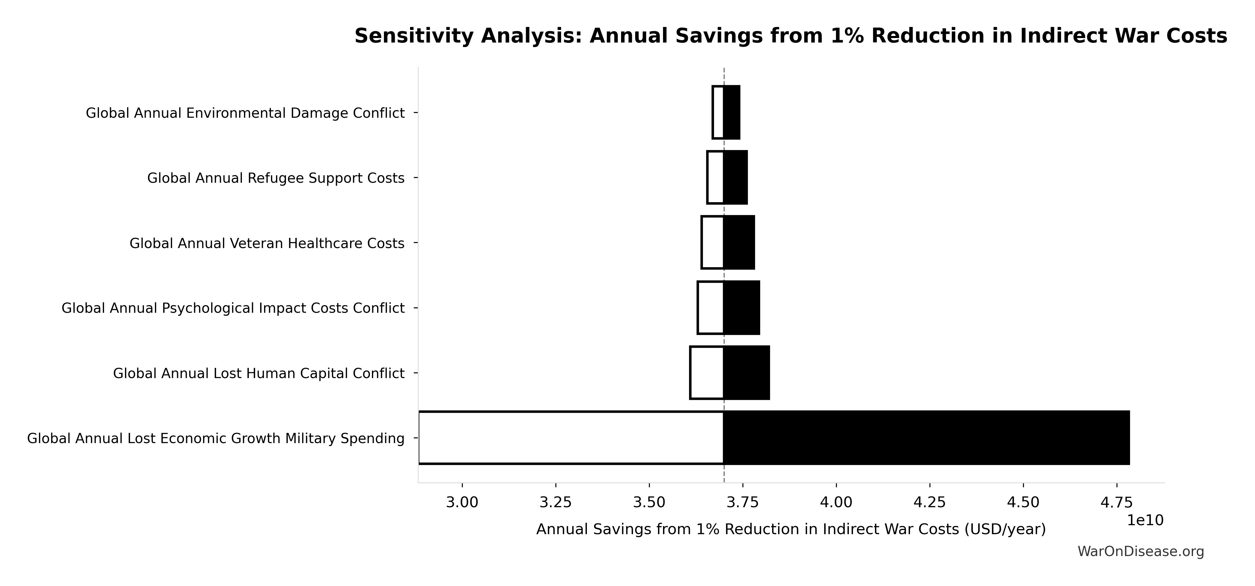
Simulation Results Summary: Total Annual Cost of War and Disease
| Statistic | Value |
|---|---|
| Baseline (deterministic) | $412T |
| Mean (expected value) | $411T |
| Median (50th percentile) | $408T |
| Standard Deviation | $106T |
| 90% Range (5th-95th percentile) | [$250T, $601T] |
The histogram shows the distribution of Total Annual Cost of War and Disease across 10,000 Monte Carlo simulations. The CDF (right) shows the probability of the outcome exceeding any given value, which is useful for risk assessment.
Exceedance Probability

This exceedance probability chart shows the likelihood that Total Annual Cost of War and Disease will exceed any given threshold. Higher curves indicate more favorable outcomes with greater certainty.
Healthcare vs Military Multiplier Ratio: 7.17x
Note📊 Details
Ratio of healthcare to military fiscal multipliers. Healthcare investment generates 7× more economic activity per dollar than military spending.
Inputs:
- Economic Multiplier for Healthcare Investment 📊: 4.3x (95% CI: 3x - 6x)
- Economic Multiplier for Military Spending 📊: 0.6x (95% CI: 0.4x - 0.9x)
\[ \begin{gathered} r_{health/mil} \\ = \frac{k_{health}}{k_{mil}} \\ = \frac{4.3}{0.6} \\ = 7.17 \end{gathered} \]
✓ High confidence
Sensitivity Analysis

Sensitivity Indices for Healthcare vs Military Multiplier Ratio
Regression-based sensitivity showing which inputs explain the most variance in the output.
| Input Parameter | Sensitivity Coefficient | Interpretation |
|---|---|---|
| Economic Multiplier for Military Spending (x) | -0.5163 | Strong driver |
| Economic Multiplier for Healthcare Investment (x) | -0.4760 | Moderate driver |
Interpretation: Standardized coefficients show the change in output (in SD units) per 1 SD change in input. Values near ±1 indicate strong influence; values exceeding ±1 may occur with correlated inputs.
Monte Carlo Distribution
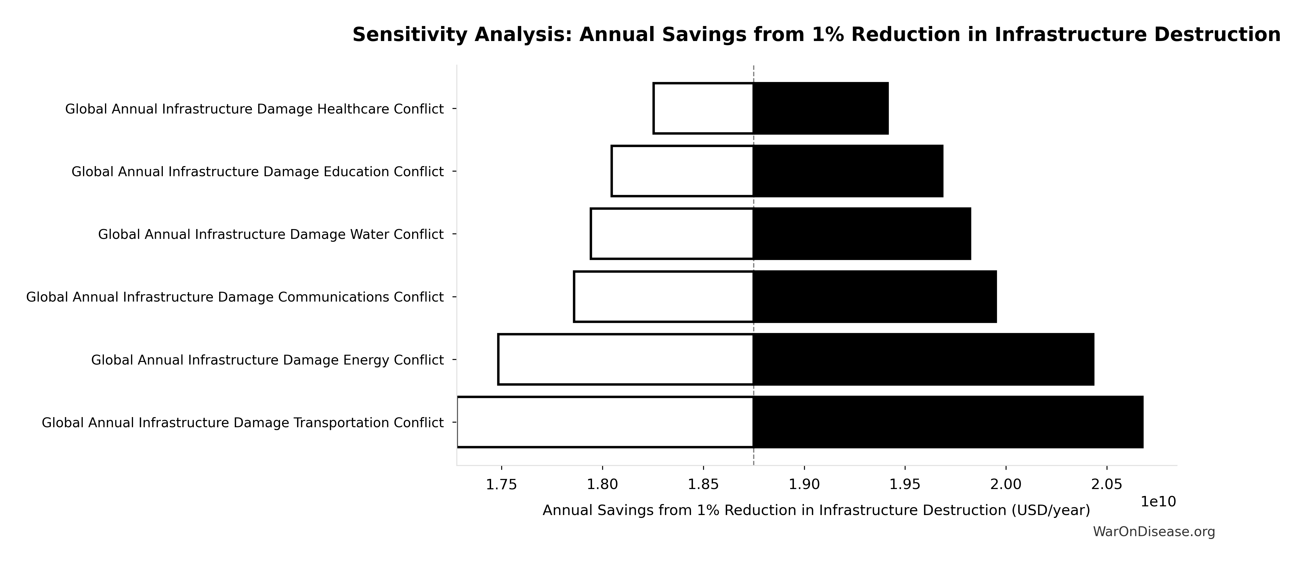
Simulation Results Summary: Healthcare vs Military Multiplier Ratio
| Statistic | Value |
|---|---|
| Baseline (deterministic) | 7.17x |
| Mean (expected value) | 7.21x |
| Median (50th percentile) | 7.22x |
| Standard Deviation | 0.227x |
| 90% Range (5th-95th percentile) | [6.83x, 7.57x] |
The histogram shows the distribution of Healthcare vs Military Multiplier Ratio across 10,000 Monte Carlo simulations. The CDF (right) shows the probability of the outcome exceeding any given value, which is useful for risk assessment.
Exceedance Probability
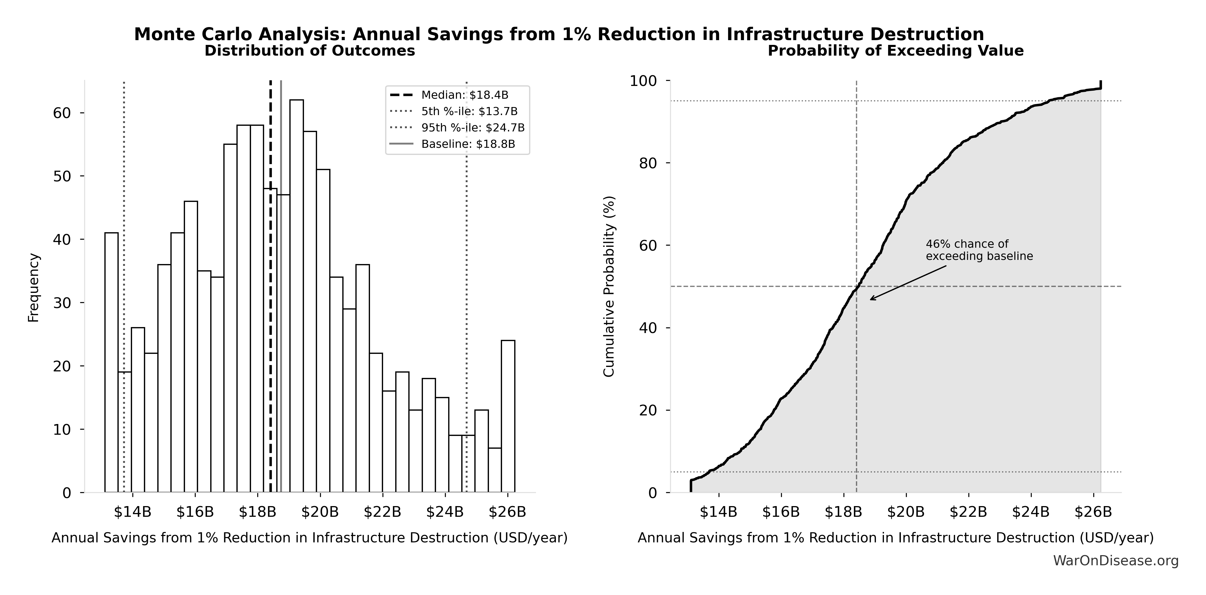
This exceedance probability chart shows the likelihood that Healthcare vs Military Multiplier Ratio will exceed any given threshold. Higher curves indicate more favorable outcomes with greater certainty.
Annual IAB Political Incentive Funding: $2.72B
Note📊 Details
Annual funding for IAB political incentive mechanism (independent expenditures supporting high-scoring politicians, post-office fellowship endowments, Public Good Score infrastructure)
Inputs:
- Annual Funding from 1% of Global Military Spending Redirected to DIH 🔢: $27.2B
- IAB Political Incentive Funding Percentage: 10%
\[ \begin{gathered} Funding_{political,ann} \\ = Funding_{treaty} \times Pct_{political} \\ = \$27.2B \times 10\% \\ = \$2.72B \end{gathered} \] where: \[ \begin{gathered} Funding_{treaty} \\ = Spending_{mil} \times Reduce_{treaty} \\ = \$2.72T \times 1\% \\ = \$27.2B \end{gathered} \] ✓ High confidence
Medical Research Spending as Percentage of Total Disease Burden: 0.0164%
Note📊 Details
Medical research spending as percentage of total disease burden
Inputs:
- Global Government Medical Research Spending 📊: $67.5B (95% CI: $54B - $81B)
- Total Annual Cost of War and Disease 🔢: $412T
\[ \begin{gathered} Pct_{RD:burden} \\ = \frac{Spending_{RD}}{Cost_{health+war}} \\ = \frac{\$67.5B}{\$412T} \\ = 0.0164\% \end{gathered} \] where: \[ \begin{gathered} Cost_{health+war} \\ = Cost_{war,total} + Burden_{disease} \\ = \$11.4T + \$400T \\ = \$412T \end{gathered} \] where: \[ \begin{gathered} Cost_{war,total} \\ = Cost_{war,direct} + Cost_{war,indirect} \\ = \$7.66T + \$3.7T \\ = \$11.4T \end{gathered} \] where: \[ \begin{gathered} Cost_{war,direct} \\ = Loss_{life,conflict} + Damage_{infra,total} \\ + Disruption_{trade} + Spending_{mil} \\ = \$2.45T + \$1.88T + \$616B + \$2.72T \\ = \$7.66T \end{gathered} \] where: \[ \begin{gathered} Loss_{life,conflict} \\ = Cost_{combat,human} + Cost_{state,human} \\ + Cost_{terror,human} \\ = \$2.34T + \$27B + \$83B \\ = \$2.45T \end{gathered} \] where: \[ \begin{gathered} Cost_{combat,human} \\ = Deaths_{combat} \times VSL \\ = 234{,}000 \times \$10M \\ = \$2.34T \end{gathered} \] where: \[ \begin{gathered} Cost_{state,human} \\ = Deaths_{state} \times VSL \\ = 2{,}700 \times \$10M \\ = \$27B \end{gathered} \] where: \[ \begin{gathered} Cost_{terror,human} \\ = Deaths_{terror} \times VSL \\ = 8{,}300 \times \$10M \\ = \$83B \end{gathered} \] where: \[ \begin{gathered} Damage_{infra,total} \\ = Damage_{comms} + Damage_{edu} + Damage_{energy} \\ + Damage_{health} + Damage_{transport} + Damage_{water} \\ = \$298B + \$234B + \$422B + \$166B + \$487B + \$268B \\ = \$1.88T \end{gathered} \] where: \[ \begin{gathered} Disruption_{trade} \\ = Disruption_{currency} + Disruption_{energy} \\ + Disruption_{shipping} + Disruption_{supply} \\ = \$57.4B + \$125B + \$247B + \$187B \\ = \$616B \end{gathered} \] where: \[ \begin{gathered} Cost_{war,indirect} \\ = Damage_{env} + Loss_{growth,mil} + Loss_{capital,conflict} \\ + Cost_{psych} + Cost_{refugee} + Cost_{vet} \\ = \$100B + \$2.72T + \$300B + \$232B + \$150B + \$200B \\ = \$3.7T \end{gathered} \] where: \[ \begin{gathered} Burden_{disease} \\ = DALYs_{global,ann} \times Pct_{avoid,DALY} \times Value_{QALY} \\ = 2.88B \times 92.6\% \times \$150K \\ = \$400T \end{gathered} \] ✓ High confidence
Sensitivity Analysis
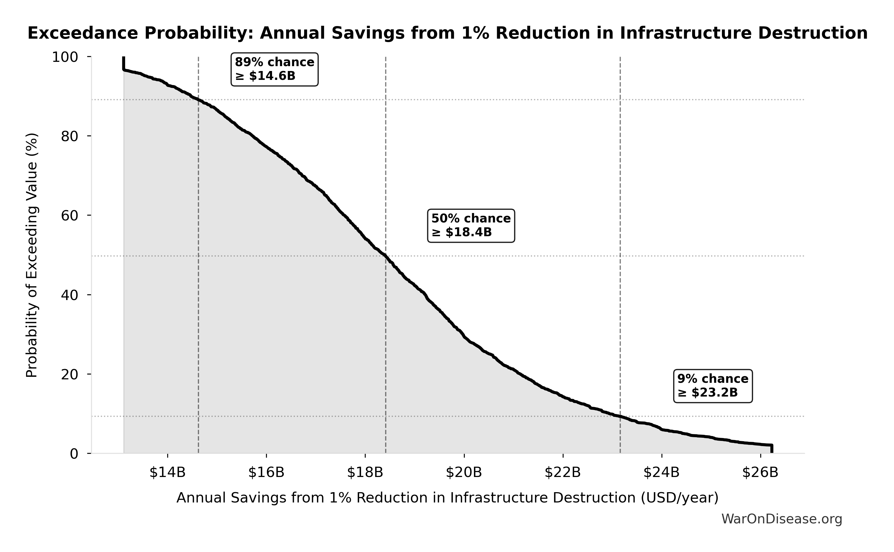
Sensitivity Indices for Medical Research Spending as Percentage of Total Disease Burden
Regression-based sensitivity showing which inputs explain the most variance in the output.
| Input Parameter | Sensitivity Coefficient | Interpretation |
|---|---|---|
| Total Annual Cost of War and Disease (USD/year) | -1.4967 | Strong driver |
| Global Government Medical Research Spending (USD) | 0.6922 | Strong driver |
Interpretation: Standardized coefficients show the change in output (in SD units) per 1 SD change in input. Values near ±1 indicate strong influence; values exceeding ±1 may occur with correlated inputs.
Monte Carlo Distribution
Simulation Results Summary: Medical Research Spending as Percentage of Total Disease Burden
| Statistic | Value |
|---|---|
| Baseline (deterministic) | 0.0164% |
| Mean (expected value) | 0.0172% |
| Median (50th percentile) | 0.0163% |
| Standard Deviation | 0.00375% |
| 90% Range (5th-95th percentile) | [0.013%, 0.0243%] |
The histogram shows the distribution of Medical Research Spending as Percentage of Total Disease Burden across 10,000 Monte Carlo simulations. The CDF (right) shows the probability of the outcome exceeding any given value, which is useful for risk assessment.
Exceedance Probability
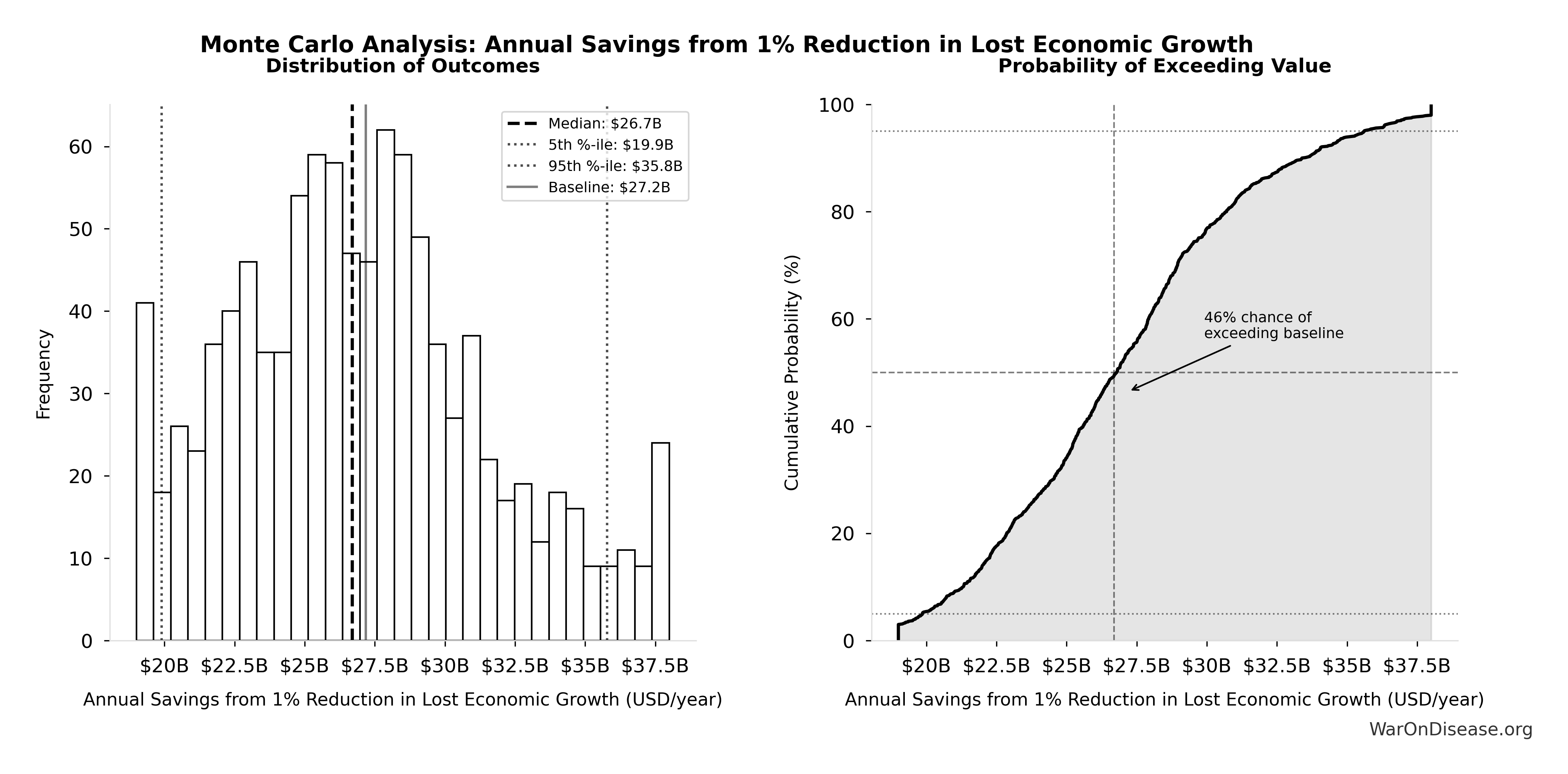
This exceedance probability chart shows the likelihood that Medical Research Spending as Percentage of Total Disease Burden will exceed any given threshold. Higher curves indicate more favorable outcomes with greater certainty.
Ratio of Military to Government Clinical Trials Spending: 604:1
Note📊 Details
Ratio of global military spending to government clinical trials spending
Inputs:
- Global Military Spending in 2024 📊: $2.72T
- Annual Global Government Spending on Clinical Trials 📊: $4.5B (95% CI: $3B - $6B)
\[ \begin{gathered} Ratio_{mil:gov} \\ = \frac{Spending_{mil}}{Spending_{trials,gov}} \\ = \frac{\$2.72T}{\$4.5B} \\ = 604 \end{gathered} \]
✓ High confidence
Sensitivity Analysis
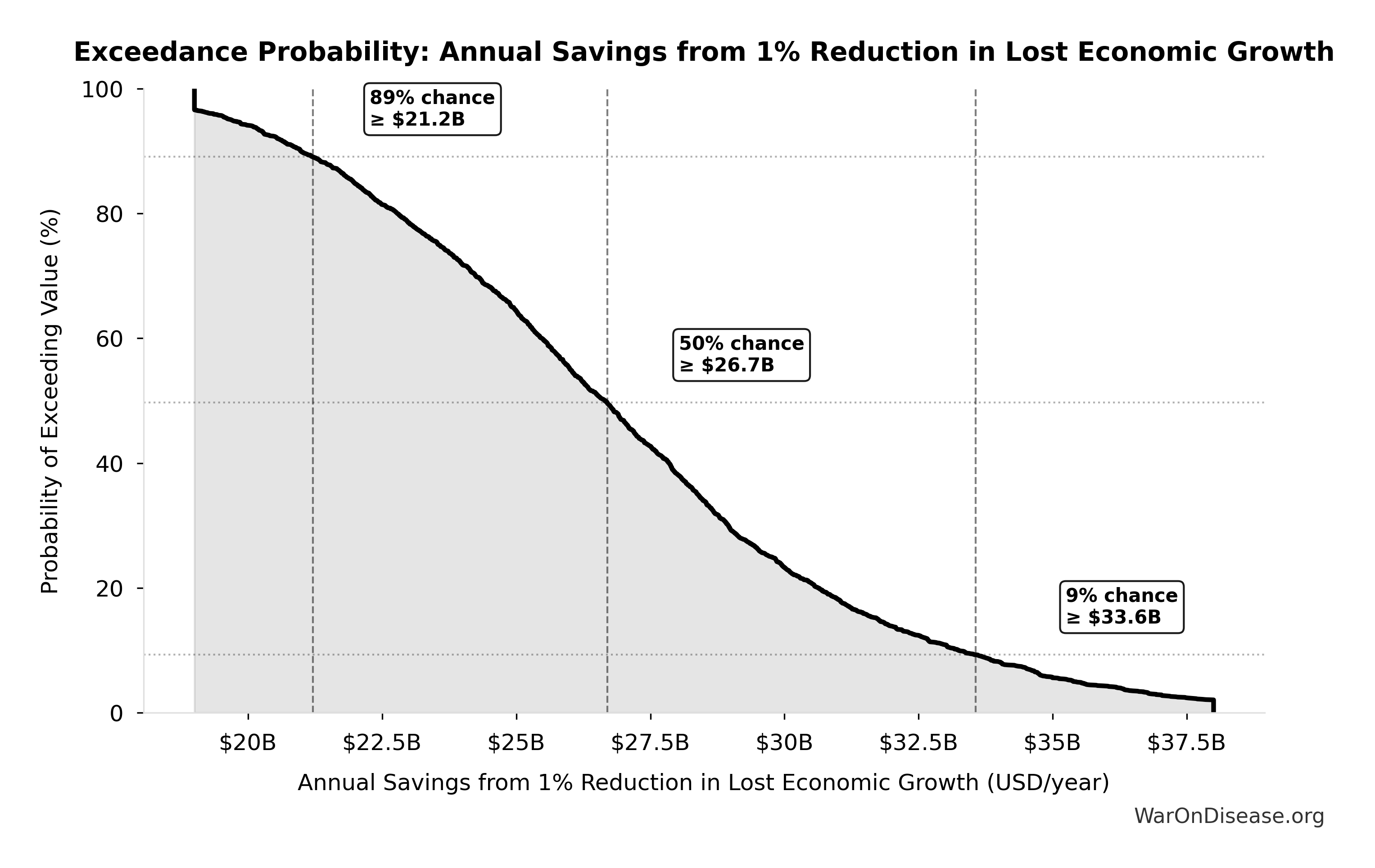
Sensitivity Indices for Ratio of Military to Government Clinical Trials Spending
Regression-based sensitivity showing which inputs explain the most variance in the output.
| Input Parameter | Sensitivity Coefficient | Interpretation |
|---|---|---|
| Annual Global Government Spending on Clinical Trials (USD) | -0.9786 | Strong driver |
Interpretation: Standardized coefficients show the change in output (in SD units) per 1 SD change in input. Values near ±1 indicate strong influence; values exceeding ±1 may occur with correlated inputs.
Monte Carlo Distribution
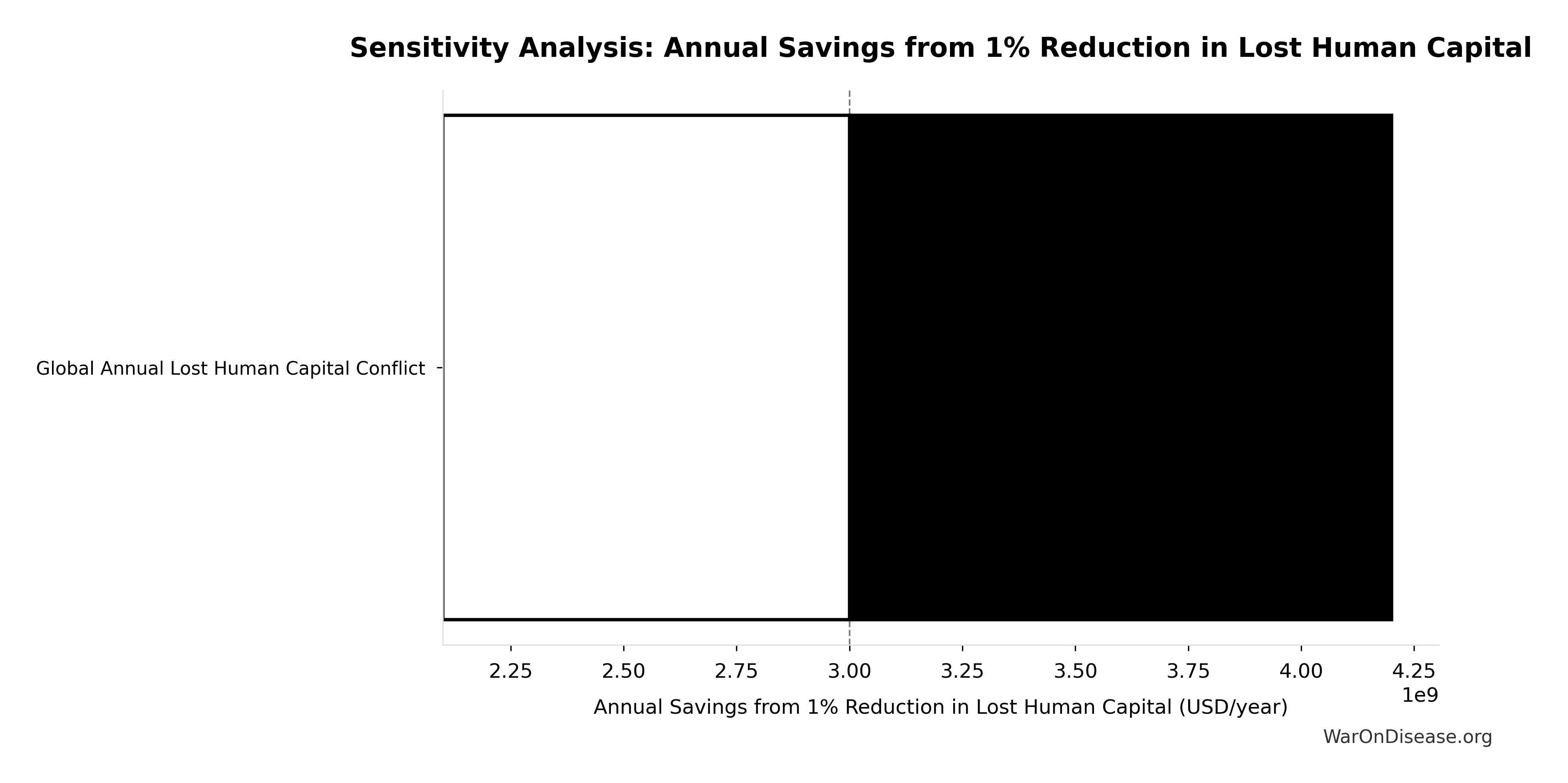
Simulation Results Summary: Ratio of Military to Government Clinical Trials Spending
| Statistic | Value |
|---|---|
| Baseline (deterministic) | 604:1 |
| Mean (expected value) | 635:1 |
| Median (50th percentile) | 621:1 |
| Standard Deviation | 127:1 |
| 90% Range (5th-95th percentile) | [453:1, 894:1] |
The histogram shows the distribution of Ratio of Military to Government Clinical Trials Spending across 10,000 Monte Carlo simulations. The CDF (right) shows the probability of the outcome exceeding any given value, which is useful for risk assessment.
Exceedance Probability
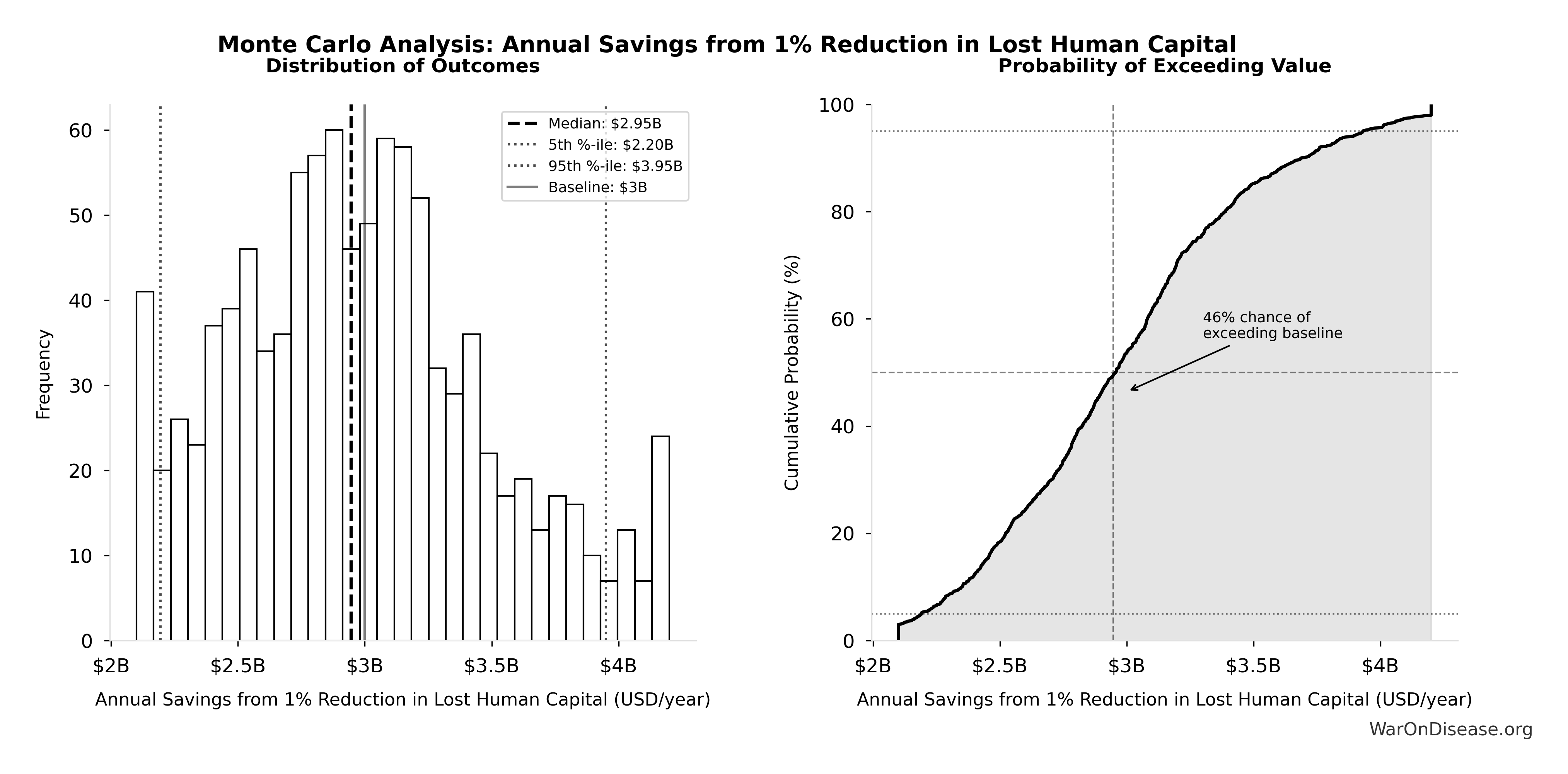
This exceedance probability chart shows the likelihood that Ratio of Military to Government Clinical Trials Spending will exceed any given threshold. Higher curves indicate more favorable outcomes with greater certainty.
Annual Peace Dividend from 1% Reduction in Total War Costs: $114B
Note📊 Details
Annual peace dividend from 1% reduction in total war costs (theoretical maximum at ε=1.0)
Inputs:
- Total Annual Cost of War Worldwide 🔢: $11.4T
- 1% Reduction in Military Spending/War Costs from Treaty: 1%
\[ \begin{gathered} Benefit_{peace,soc} \\ = Cost_{war,total} \times Reduce_{treaty} \\ = \$11.4T \times 1\% \\ = \$114B \end{gathered} \] where: \[ \begin{gathered} Cost_{war,total} \\ = Cost_{war,direct} + Cost_{war,indirect} \\ = \$7.66T + \$3.7T \\ = \$11.4T \end{gathered} \] where: \[ \begin{gathered} Cost_{war,direct} \\ = Loss_{life,conflict} + Damage_{infra,total} \\ + Disruption_{trade} + Spending_{mil} \\ = \$2.45T + \$1.88T + \$616B + \$2.72T \\ = \$7.66T \end{gathered} \] where: \[ \begin{gathered} Loss_{life,conflict} \\ = Cost_{combat,human} + Cost_{state,human} \\ + Cost_{terror,human} \\ = \$2.34T + \$27B + \$83B \\ = \$2.45T \end{gathered} \] where: \[ \begin{gathered} Cost_{combat,human} \\ = Deaths_{combat} \times VSL \\ = 234{,}000 \times \$10M \\ = \$2.34T \end{gathered} \] where: \[ \begin{gathered} Cost_{state,human} \\ = Deaths_{state} \times VSL \\ = 2{,}700 \times \$10M \\ = \$27B \end{gathered} \] where: \[ \begin{gathered} Cost_{terror,human} \\ = Deaths_{terror} \times VSL \\ = 8{,}300 \times \$10M \\ = \$83B \end{gathered} \] where: \[ \begin{gathered} Damage_{infra,total} \\ = Damage_{comms} + Damage_{edu} + Damage_{energy} \\ + Damage_{health} + Damage_{transport} + Damage_{water} \\ = \$298B + \$234B + \$422B + \$166B + \$487B + \$268B \\ = \$1.88T \end{gathered} \] where: \[ \begin{gathered} Disruption_{trade} \\ = Disruption_{currency} + Disruption_{energy} \\ + Disruption_{shipping} + Disruption_{supply} \\ = \$57.4B + \$125B + \$247B + \$187B \\ = \$616B \end{gathered} \] where: \[ \begin{gathered} Cost_{war,indirect} \\ = Damage_{env} + Loss_{growth,mil} + Loss_{capital,conflict} \\ + Cost_{psych} + Cost_{refugee} + Cost_{vet} \\ = \$100B + \$2.72T + \$300B + \$232B + \$150B + \$200B \\ = \$3.7T \end{gathered} \] ✓ High confidence
Sensitivity Analysis
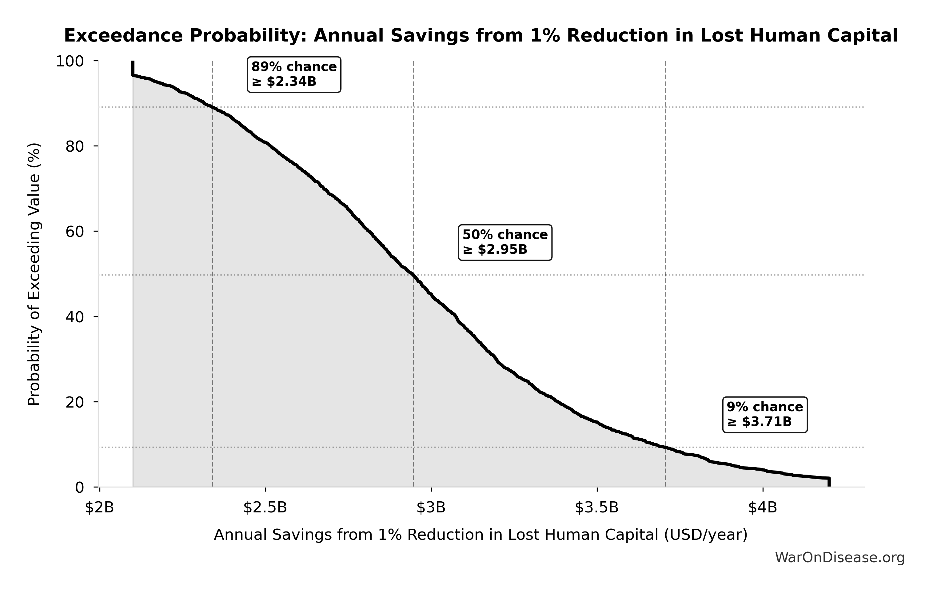
Sensitivity Indices for Annual Peace Dividend from 1% Reduction in Total War Costs
Regression-based sensitivity showing which inputs explain the most variance in the output.
| Input Parameter | Sensitivity Coefficient | Interpretation |
|---|---|---|
| Total Annual Cost of War Worldwide (USD/year) | 1.0000 | Strong driver |
Interpretation: Standardized coefficients show the change in output (in SD units) per 1 SD change in input. Values near ±1 indicate strong influence; values exceeding ±1 may occur with correlated inputs.
Monte Carlo Distribution
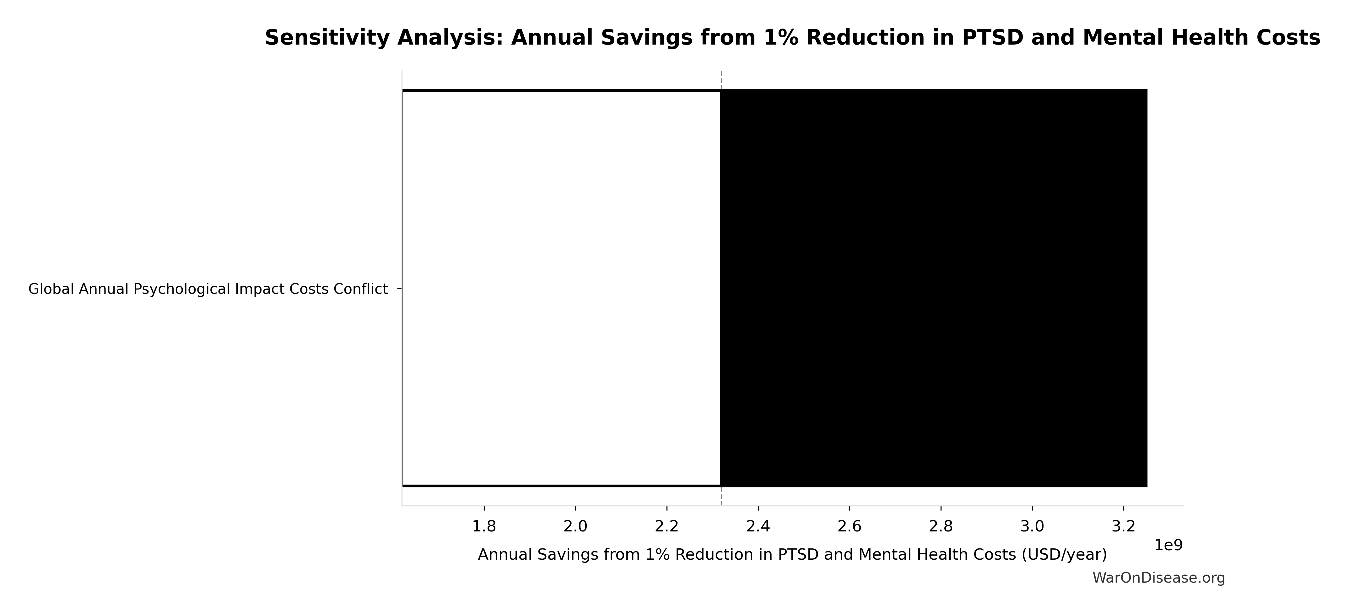
Simulation Results Summary: Annual Peace Dividend from 1% Reduction in Total War Costs
| Statistic | Value |
|---|---|
| Baseline (deterministic) | $114B |
| Mean (expected value) | $113B |
| Median (50th percentile) | $112B |
| Standard Deviation | $15.1B |
| 90% Range (5th-95th percentile) | [$90.1B, $141B] |
The histogram shows the distribution of Annual Peace Dividend from 1% Reduction in Total War Costs across 10,000 Monte Carlo simulations. The CDF (right) shows the probability of the outcome exceeding any given value, which is useful for risk assessment.
Exceedance Probability
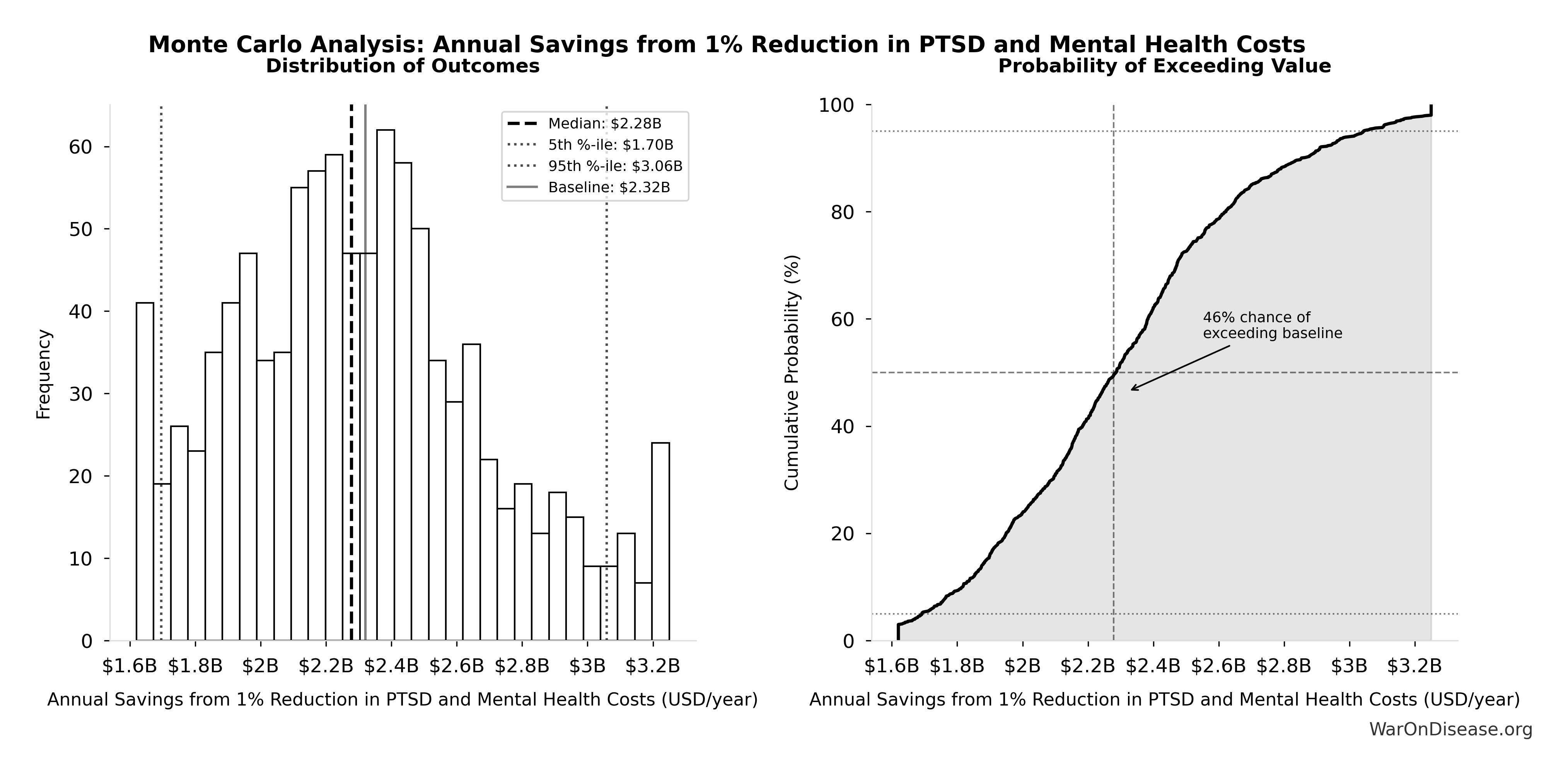
This exceedance probability chart shows the likelihood that Annual Peace Dividend from 1% Reduction in Total War Costs will exceed any given threshold. Higher curves indicate more favorable outcomes with greater certainty.
Conflict Reduction Benefits from 1% Less Military Spending: $86.4B
Note📊 Details
Conflict reduction benefits from 1% less military spending (lower confidence - assumes proportional relationship)
Inputs:
- Annual Peace Dividend from 1% Reduction in Total War Costs 🔢: $114B
- Annual Funding from 1% of Global Military Spending Redirected to DIH 🔢: $27.2B
\[ \begin{gathered} Savings_{conflict} \\ = Benefit_{peace,soc} - Funding_{treaty} \\ = \$114B - \$27.2B \\ = \$86.4B \end{gathered} \] where: \[ \begin{gathered} Benefit_{peace,soc} \\ = Cost_{war,total} \times Reduce_{treaty} \\ = \$11.4T \times 1\% \\ = \$114B \end{gathered} \] where: \[ \begin{gathered} Cost_{war,total} \\ = Cost_{war,direct} + Cost_{war,indirect} \\ = \$7.66T + \$3.7T \\ = \$11.4T \end{gathered} \] where: \[ \begin{gathered} Cost_{war,direct} \\ = Loss_{life,conflict} + Damage_{infra,total} \\ + Disruption_{trade} + Spending_{mil} \\ = \$2.45T + \$1.88T + \$616B + \$2.72T \\ = \$7.66T \end{gathered} \] where: \[ \begin{gathered} Loss_{life,conflict} \\ = Cost_{combat,human} + Cost_{state,human} \\ + Cost_{terror,human} \\ = \$2.34T + \$27B + \$83B \\ = \$2.45T \end{gathered} \] where: \[ \begin{gathered} Cost_{combat,human} \\ = Deaths_{combat} \times VSL \\ = 234{,}000 \times \$10M \\ = \$2.34T \end{gathered} \] where: \[ \begin{gathered} Cost_{state,human} \\ = Deaths_{state} \times VSL \\ = 2{,}700 \times \$10M \\ = \$27B \end{gathered} \] where: \[ \begin{gathered} Cost_{terror,human} \\ = Deaths_{terror} \times VSL \\ = 8{,}300 \times \$10M \\ = \$83B \end{gathered} \] where: \[ \begin{gathered} Damage_{infra,total} \\ = Damage_{comms} + Damage_{edu} + Damage_{energy} \\ + Damage_{health} + Damage_{transport} + Damage_{water} \\ = \$298B + \$234B + \$422B + \$166B + \$487B + \$268B \\ = \$1.88T \end{gathered} \] where: \[ \begin{gathered} Disruption_{trade} \\ = Disruption_{currency} + Disruption_{energy} \\ + Disruption_{shipping} + Disruption_{supply} \\ = \$57.4B + \$125B + \$247B + \$187B \\ = \$616B \end{gathered} \] where: \[ \begin{gathered} Cost_{war,indirect} \\ = Damage_{env} + Loss_{growth,mil} + Loss_{capital,conflict} \\ + Cost_{psych} + Cost_{refugee} + Cost_{vet} \\ = \$100B + \$2.72T + \$300B + \$232B + \$150B + \$200B \\ = \$3.7T \end{gathered} \] where: \[ \begin{gathered} Funding_{treaty} \\ = Spending_{mil} \times Reduce_{treaty} \\ = \$2.72T \times 1\% \\ = \$27.2B \end{gathered} \] Methodology: Direct Calculation
? Low confidence
Sensitivity Analysis
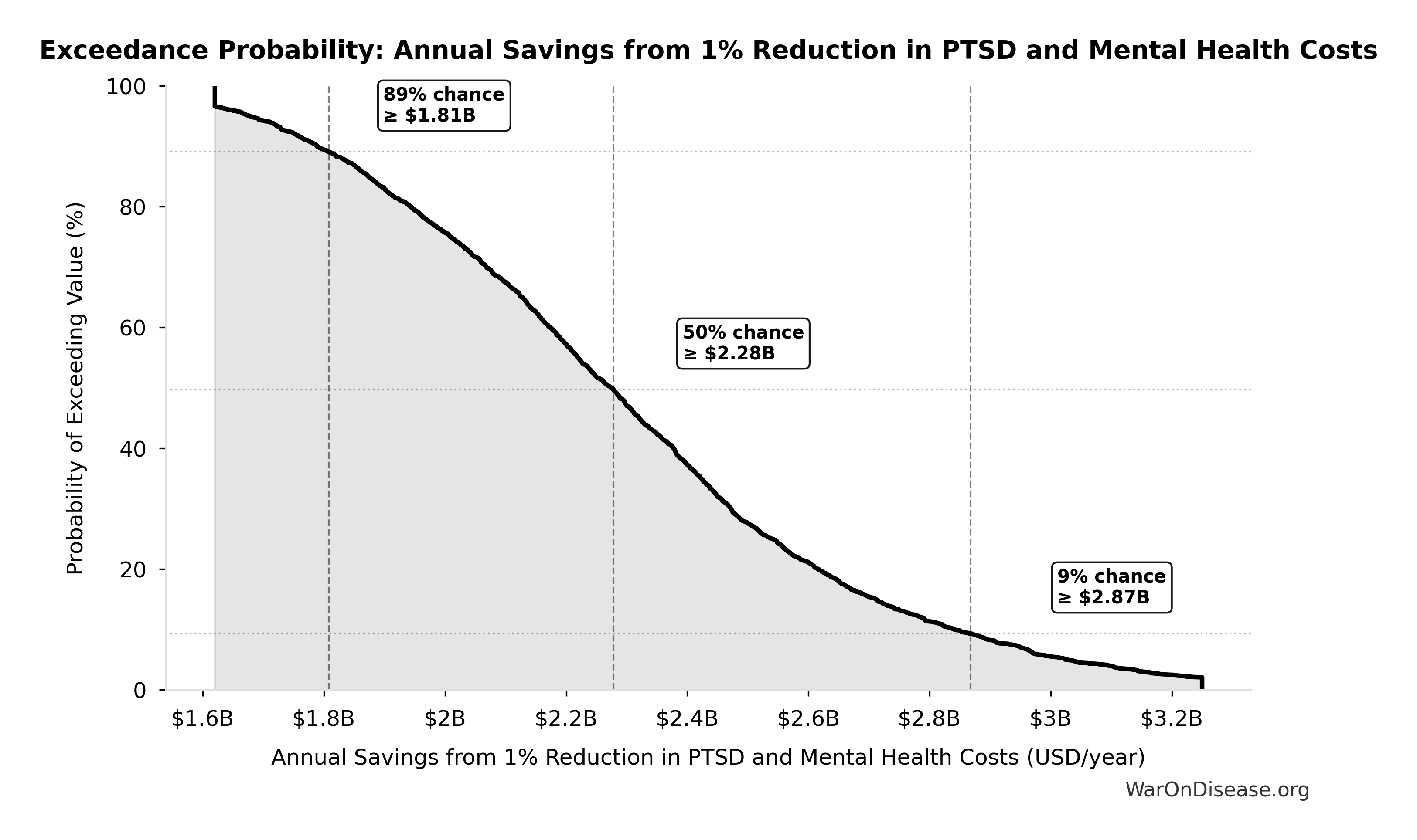
Sensitivity Indices for Conflict Reduction Benefits from 1% Less Military Spending
Regression-based sensitivity showing which inputs explain the most variance in the output.
| Input Parameter | Sensitivity Coefficient | Interpretation |
|---|---|---|
| Annual Peace Dividend from 1% Reduction in Total War Costs (USD/year) | 1.0000 | Strong driver |
Interpretation: Standardized coefficients show the change in output (in SD units) per 1 SD change in input. Values near ±1 indicate strong influence; values exceeding ±1 may occur with correlated inputs.
Monte Carlo Distribution
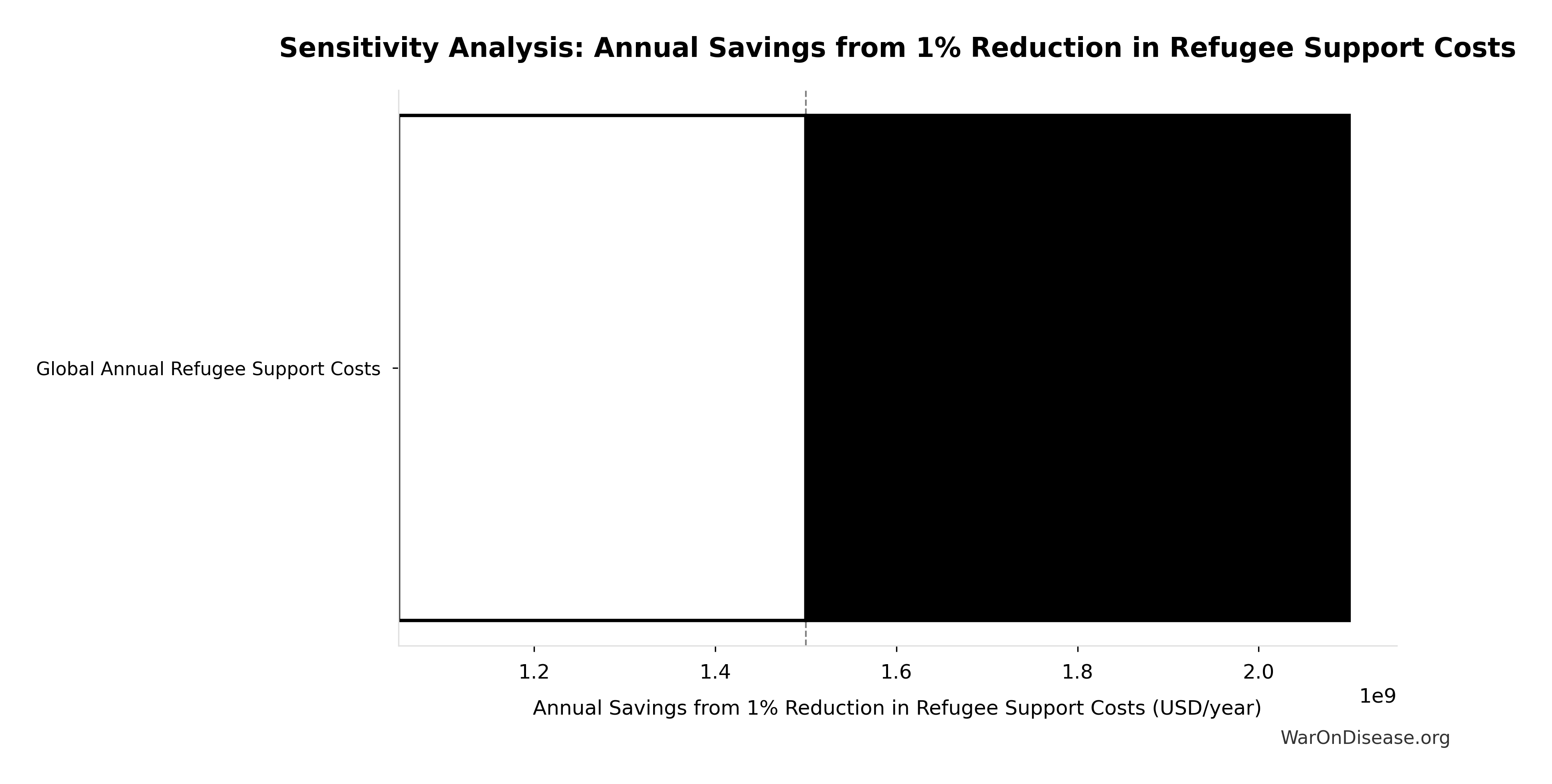
Simulation Results Summary: Conflict Reduction Benefits from 1% Less Military Spending
| Statistic | Value |
|---|---|
| Baseline (deterministic) | $86.4B |
| Mean (expected value) | $85.9B |
| Median (50th percentile) | $84.6B |
| Standard Deviation | $15.1B |
| 90% Range (5th-95th percentile) | [$62.9B, $113B] |
The histogram shows the distribution of Conflict Reduction Benefits from 1% Less Military Spending across 10,000 Monte Carlo simulations. The CDF (right) shows the probability of the outcome exceeding any given value, which is useful for risk assessment.
Exceedance Probability
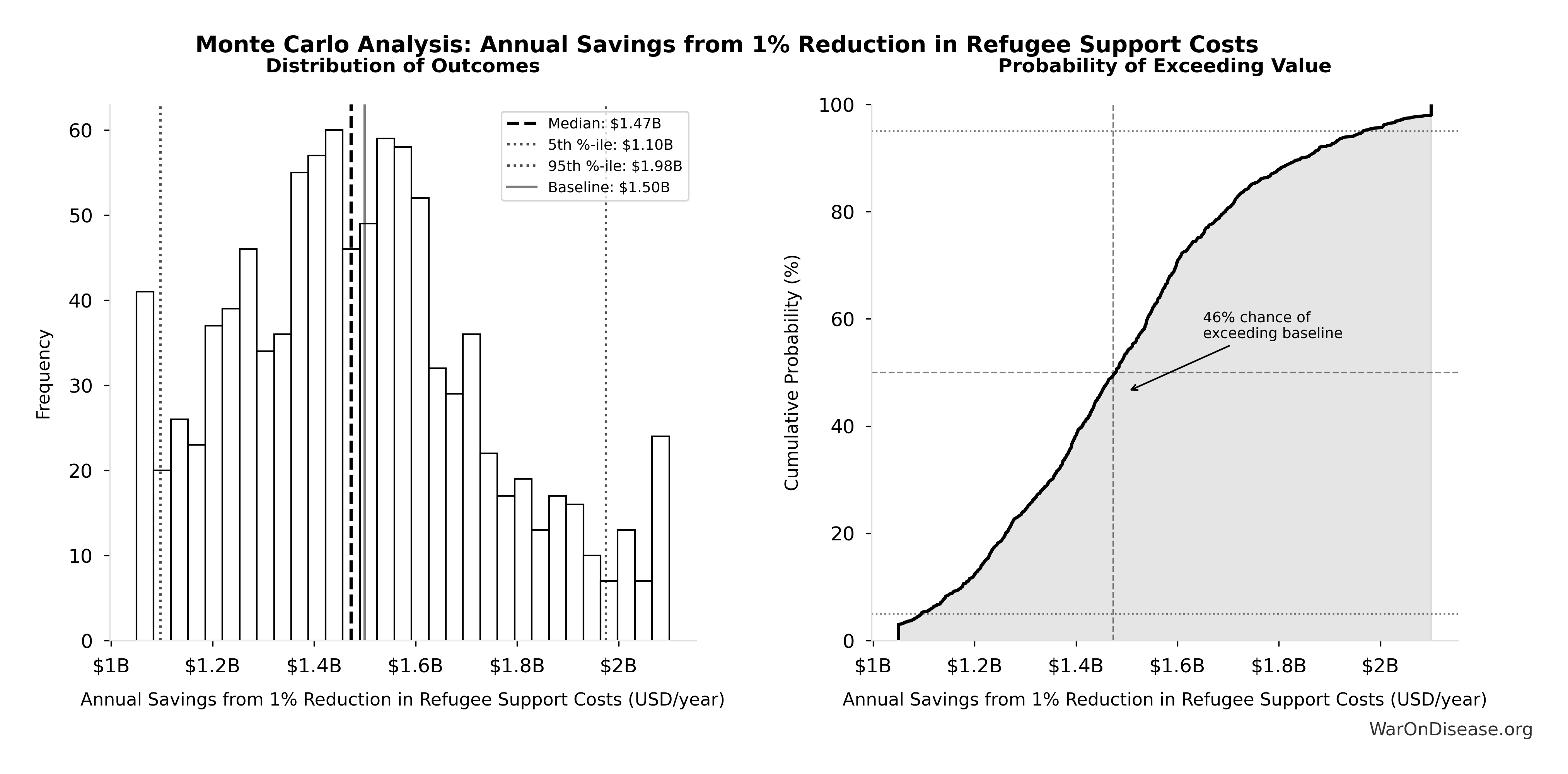
This exceedance probability chart shows the likelihood that Conflict Reduction Benefits from 1% Less Military Spending will exceed any given threshold. Higher curves indicate more favorable outcomes with greater certainty.
Percentage Military Spending Cut After WW2: 87.6%
Note📊 Details
Percentage US military spending cut after WW2 (1945-1947, inflation-adjusted: $1,420B to $176B in constant 2024 dollars)
Inputs:
- US Military Spending in 1947 (Constant 2024 Dollars) 📊: $176B
- US Military Spending at WW2 Peak (Constant 2024 Dollars) 📊: $1.42T
\[ \begin{gathered} Cut_{WW2} \\ = 1 - \frac{Spending_{US,1947}}{Spending_{US,1945}} \\ = 1 - \frac{\$176B}{\$1.42T} \\ = 87.6\% \end{gathered} \]
✓ High confidence
Pragmatic Trial Cost per QALY (RECOVERY): $4
Note📊 Details
Cost per QALY for pragmatic platform trials, calculated from RECOVERY trial data. Uses global impact methodology: trial cost divided by total QALYs from downstream adoption. This measures research efficiency (discovery value), not clinical intervention ICER.
Inputs:
- RECOVERY Trial Total Cost 📊: $20M (95% CI: $15M - $25M)
- RECOVERY Trial Total QALYs Generated 🔢: 5 million QALYs
\[ \begin{gathered} Cost_{pragmatic,QALY} \\ = \frac{Cost_{RECOVERY}}{QALY_{RECOVERY}} \\ = \frac{\$20M}{5M} \\ = \$4 \end{gathered} \] where: \[ \begin{gathered} QALY_{RECOVERY} \\ = Lives_{RECOVERY} \times QALY_{COVID} \\ = 1M \times 5 \\ = 5M \end{gathered} \] Methodology:72
~ Medium confidence
Sensitivity Analysis
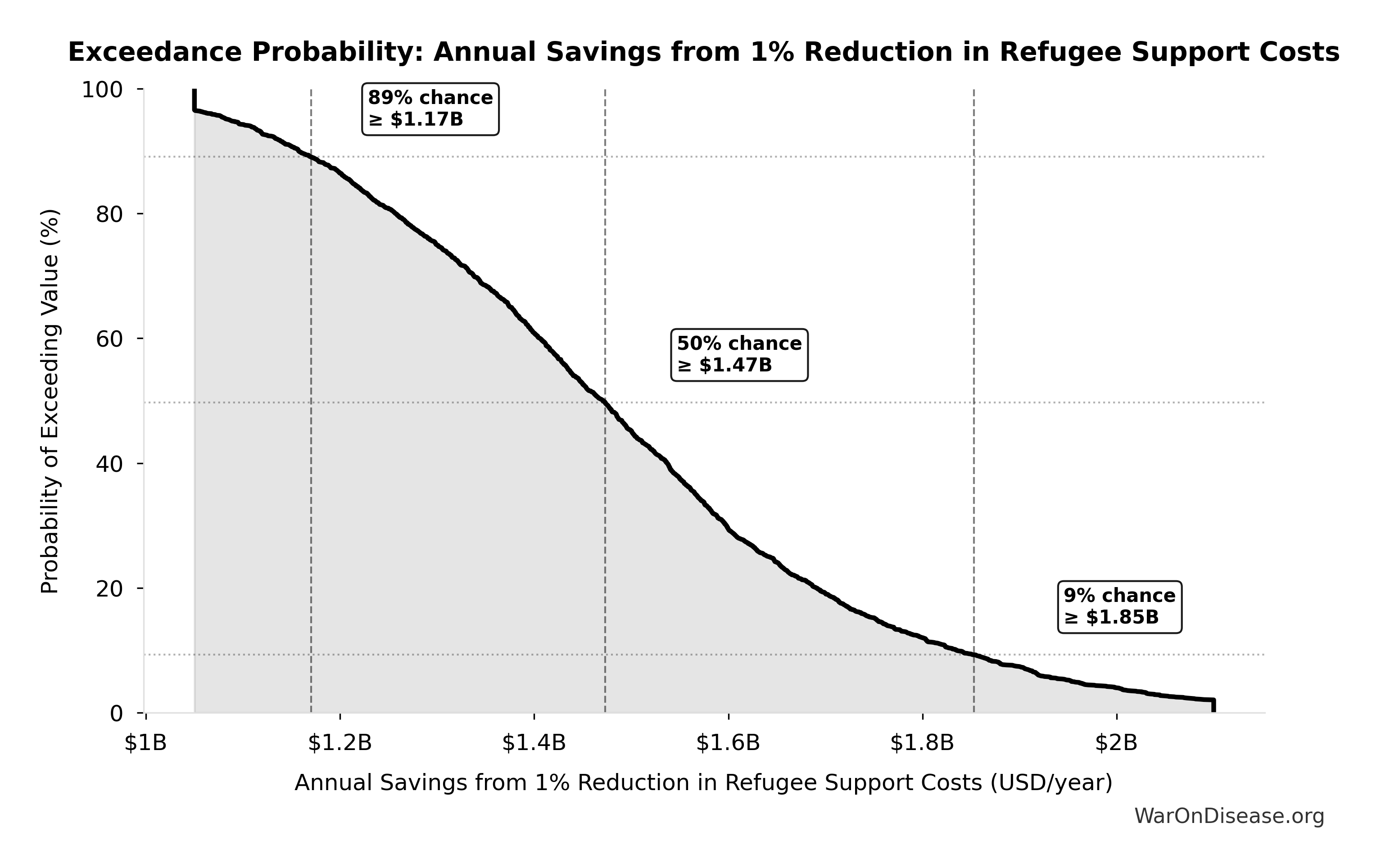
Sensitivity Indices for Pragmatic Trial Cost per QALY (RECOVERY)
Regression-based sensitivity showing which inputs explain the most variance in the output.
| Input Parameter | Sensitivity Coefficient | Interpretation |
|---|---|---|
| RECOVERY Trial Total Cost (USD) | -1.4871 | Strong driver |
| RECOVERY Trial Total QALYs Generated (QALYs) | 0.5682 | Strong driver |
Interpretation: Standardized coefficients show the change in output (in SD units) per 1 SD change in input. Values near ±1 indicate strong influence; values exceeding ±1 may occur with correlated inputs.
Monte Carlo Distribution
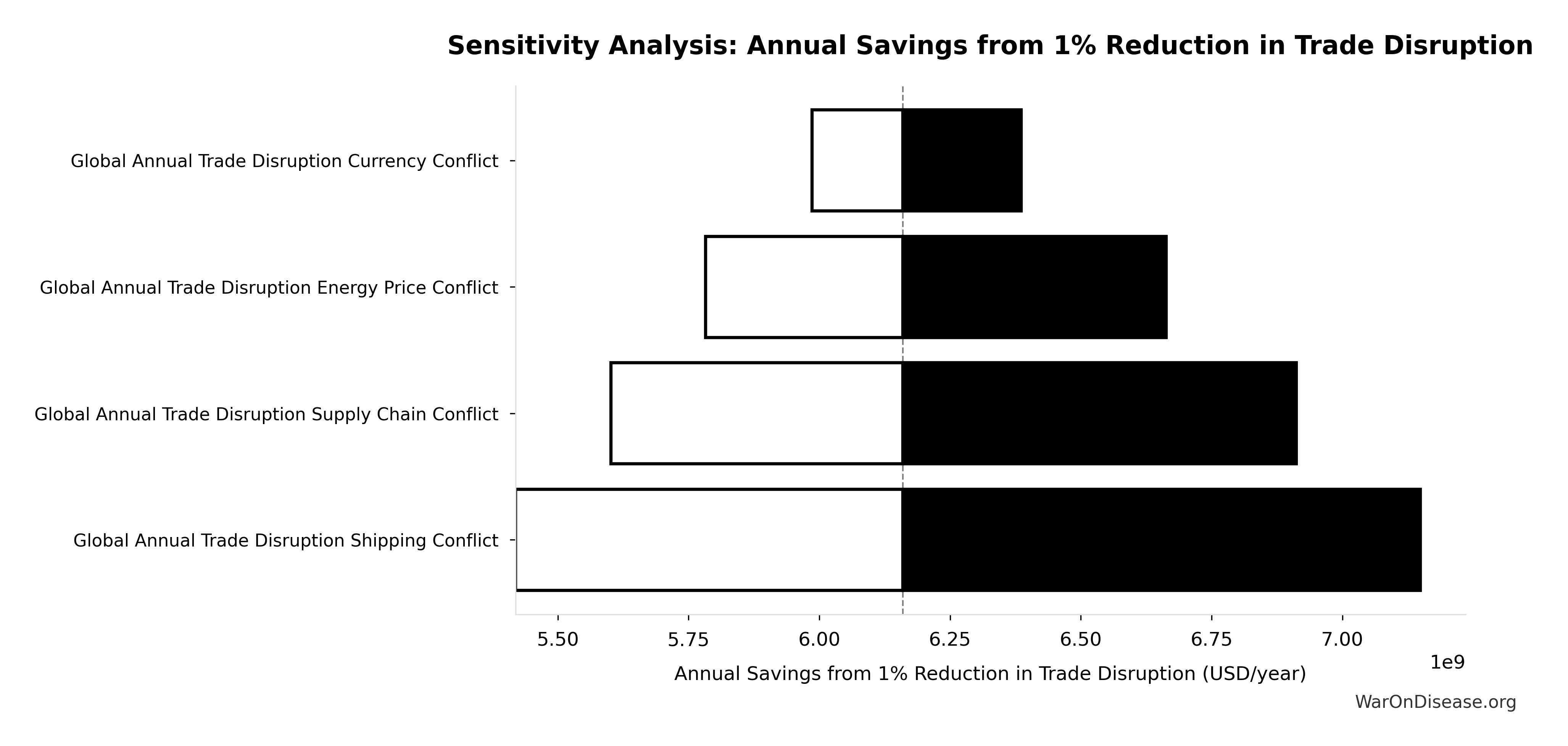
Simulation Results Summary: Pragmatic Trial Cost per QALY (RECOVERY)
| Statistic | Value |
|---|---|
| Baseline (deterministic) | $4 |
| Mean (expected value) | $5.1 |
| Median (50th percentile) | $4.55 |
| Standard Deviation | $2.59 |
| 90% Range (5th-95th percentile) | [$1.71, $10] |
The histogram shows the distribution of Pragmatic Trial Cost per QALY (RECOVERY) across 10,000 Monte Carlo simulations. The CDF (right) shows the probability of the outcome exceeding any given value, which is useful for risk assessment.
Exceedance Probability
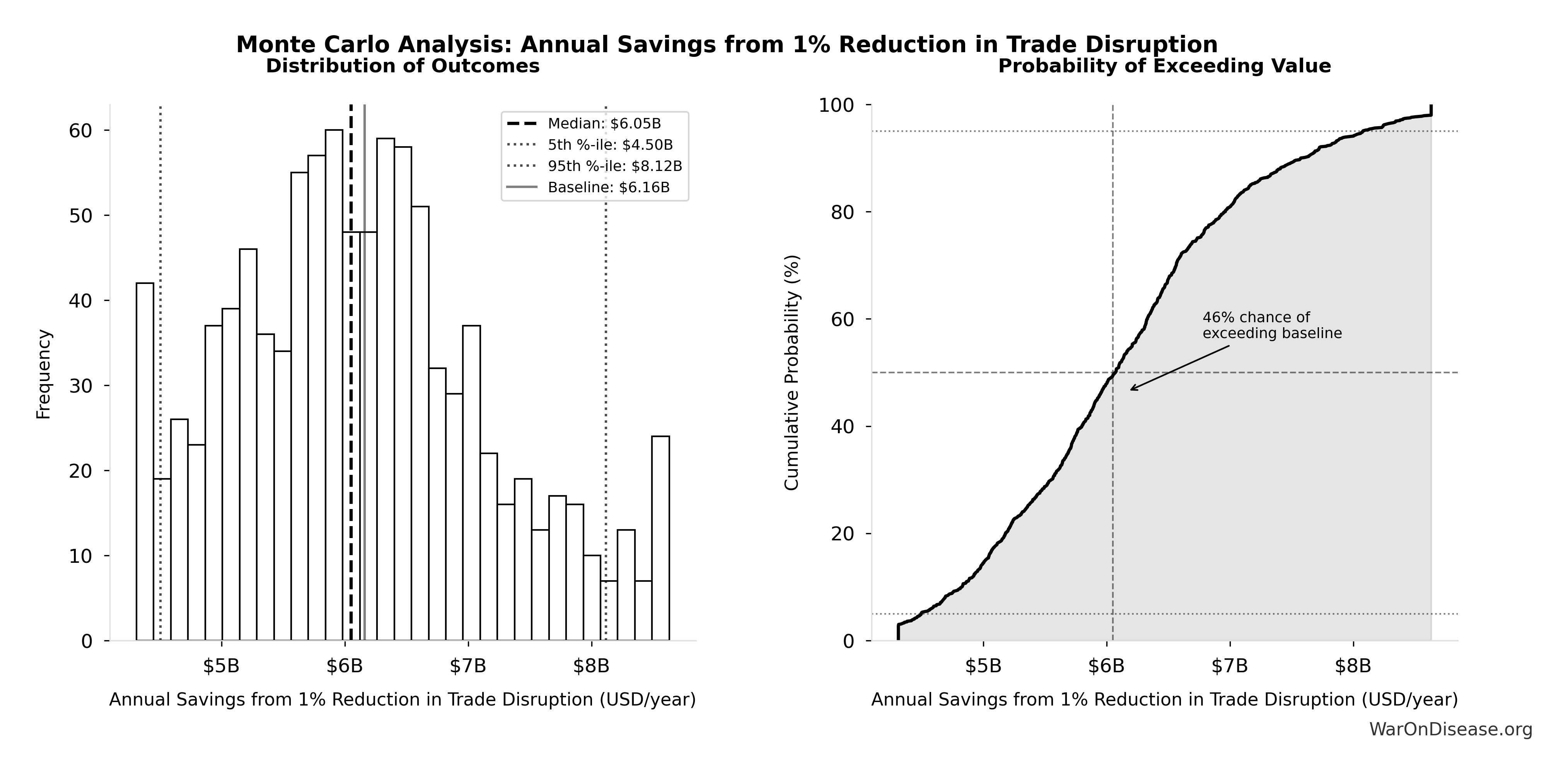
This exceedance probability chart shows the likelihood that Pragmatic Trial Cost per QALY (RECOVERY) will exceed any given threshold. Higher curves indicate more favorable outcomes with greater certainty.
RECOVERY Trial Cost Reduction Factor: 82x
Note📊 Details
Cost reduction factor demonstrated by RECOVERY trial (traditional Phase 3 cost / RECOVERY cost per patient)
Inputs:
- Phase 3 Cost per Patient 📊: $41K (95% CI: $20K - $120K)
- Recovery Trial Cost per Patient 📊: $500 (95% CI: $400 - $2.5K)
\[ \begin{gathered} k_{RECOVERY} \\ = \frac{Cost_{P3,pt}}{Cost_{RECOVERY,pt}} \\ = \frac{\$41K}{\$500} \\ = 82 \end{gathered} \]
Methodology:72
✓ High confidence
Sensitivity Analysis
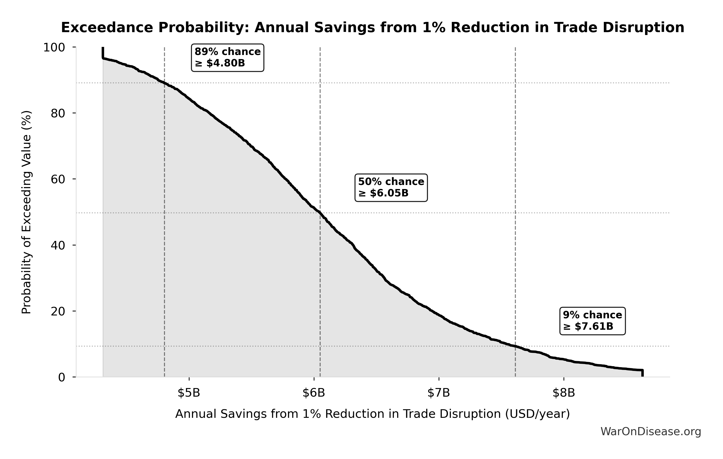
Sensitivity Indices for RECOVERY Trial Cost Reduction Factor
Regression-based sensitivity showing which inputs explain the most variance in the output.
| Input Parameter | Sensitivity Coefficient | Interpretation |
|---|---|---|
| Recovery Trial Cost per Patient (USD/patient) | -2.4783 | Strong driver |
| Phase 3 Cost per Patient (USD/patient) | 2.4635 | Strong driver |
Interpretation: Standardized coefficients show the change in output (in SD units) per 1 SD change in input. Values near ±1 indicate strong influence; values exceeding ±1 may occur with correlated inputs.
Monte Carlo Distribution
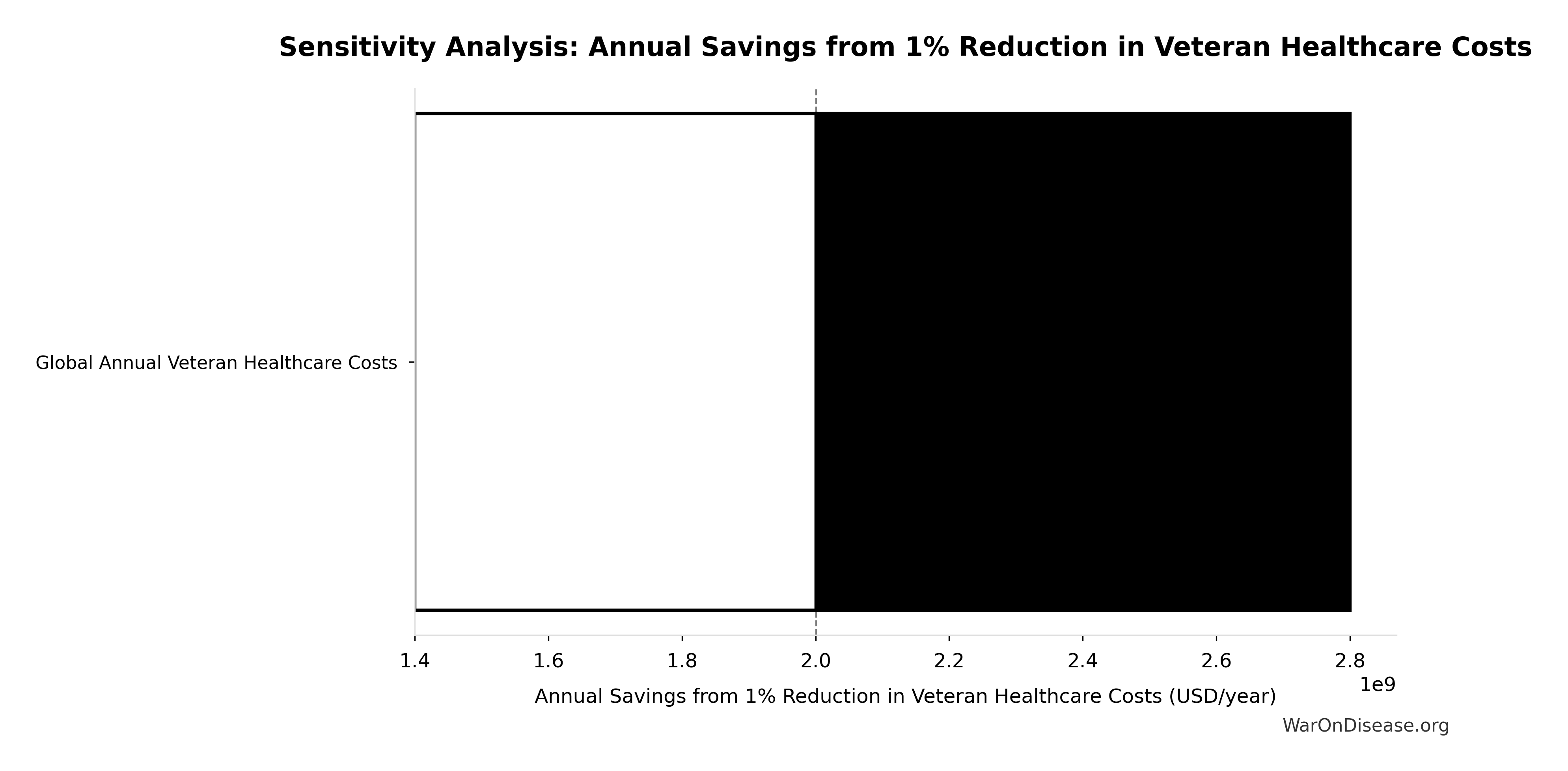
Simulation Results Summary: RECOVERY Trial Cost Reduction Factor
| Statistic | Value |
|---|---|
| Baseline (deterministic) | 82x |
| Mean (expected value) | 71.2x |
| Median (50th percentile) | 72.4x |
| Standard Deviation | 15.3x |
| 90% Range (5th-95th percentile) | [50x, 94.1x] |
The histogram shows the distribution of RECOVERY Trial Cost Reduction Factor across 10,000 Monte Carlo simulations. The CDF (right) shows the probability of the outcome exceeding any given value, which is useful for risk assessment.
Exceedance Probability
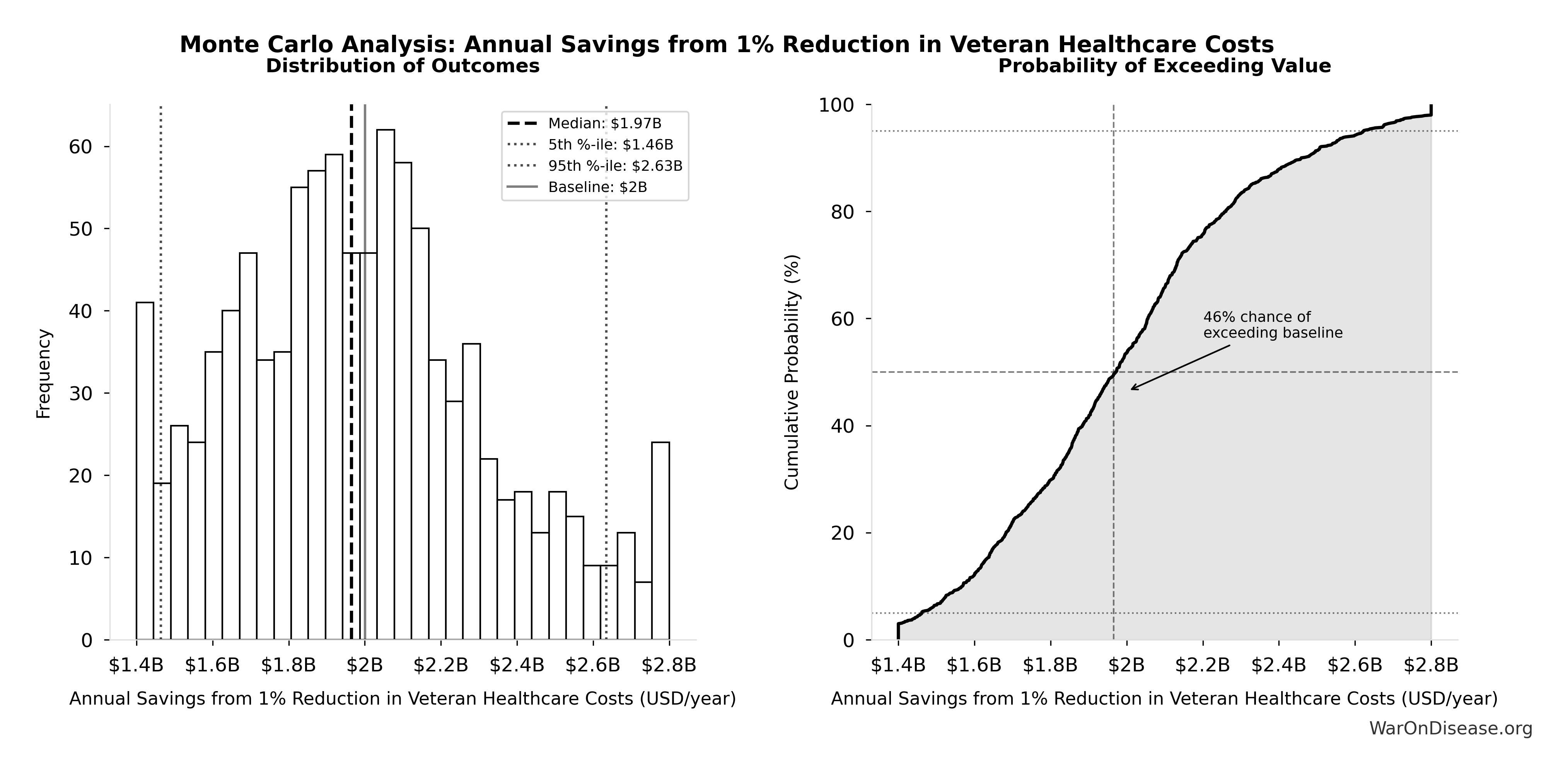
This exceedance probability chart shows the likelihood that RECOVERY Trial Cost Reduction Factor will exceed any given threshold. Higher curves indicate more favorable outcomes with greater certainty.
RECOVERY Trial Total QALYs Generated: 5 million QALYs
Note📊 Details
Total QALYs generated by RECOVERY trial’s discoveries (lives saved × QALYs per life). Uses global impact methodology: counts all downstream health gains from the discovery.
Inputs:
- RECOVERY Trial Global Lives Saved 📊: 1 million lives (95% CI: 500 thousand lives - 2 million lives)
- QALYs per COVID Death Averted: 5 QALYs/death (95% CI: 3 QALYs/death - 10 QALYs/death)
\[ \begin{gathered} QALY_{RECOVERY} \\ = Lives_{RECOVERY} \times QALY_{COVID} \\ = 1M \times 5 \\ = 5M \end{gathered} \]
~ Medium confidence
Sensitivity Analysis
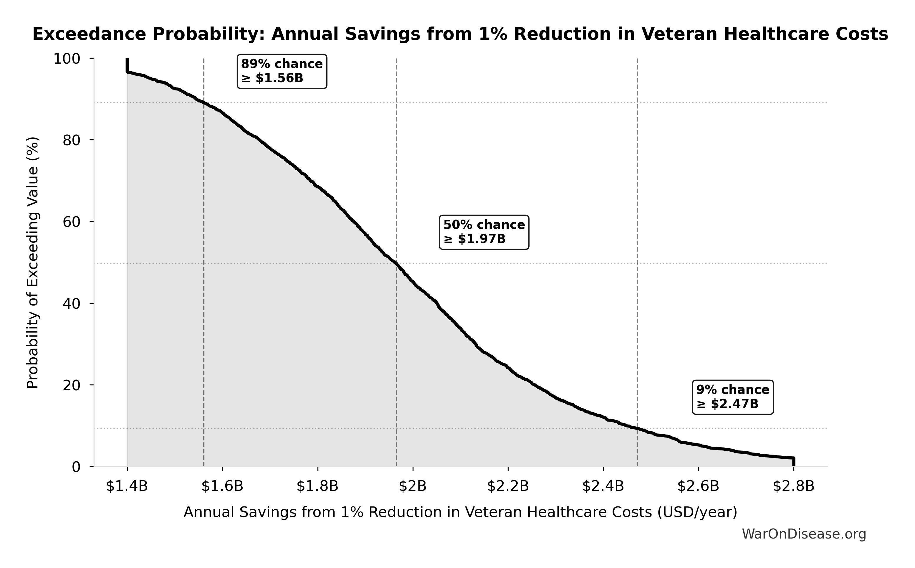
Sensitivity Indices for RECOVERY Trial Total QALYs Generated
Regression-based sensitivity showing which inputs explain the most variance in the output.
| Input Parameter | Sensitivity Coefficient | Interpretation |
|---|---|---|
| QALYs per COVID Death Averted (QALYs/death) | 2.2404 | Strong driver |
| RECOVERY Trial Global Lives Saved (lives) | -1.2571 | Strong driver |
Interpretation: Standardized coefficients show the change in output (in SD units) per 1 SD change in input. Values near ±1 indicate strong influence; values exceeding ±1 may occur with correlated inputs.
Monte Carlo Distribution
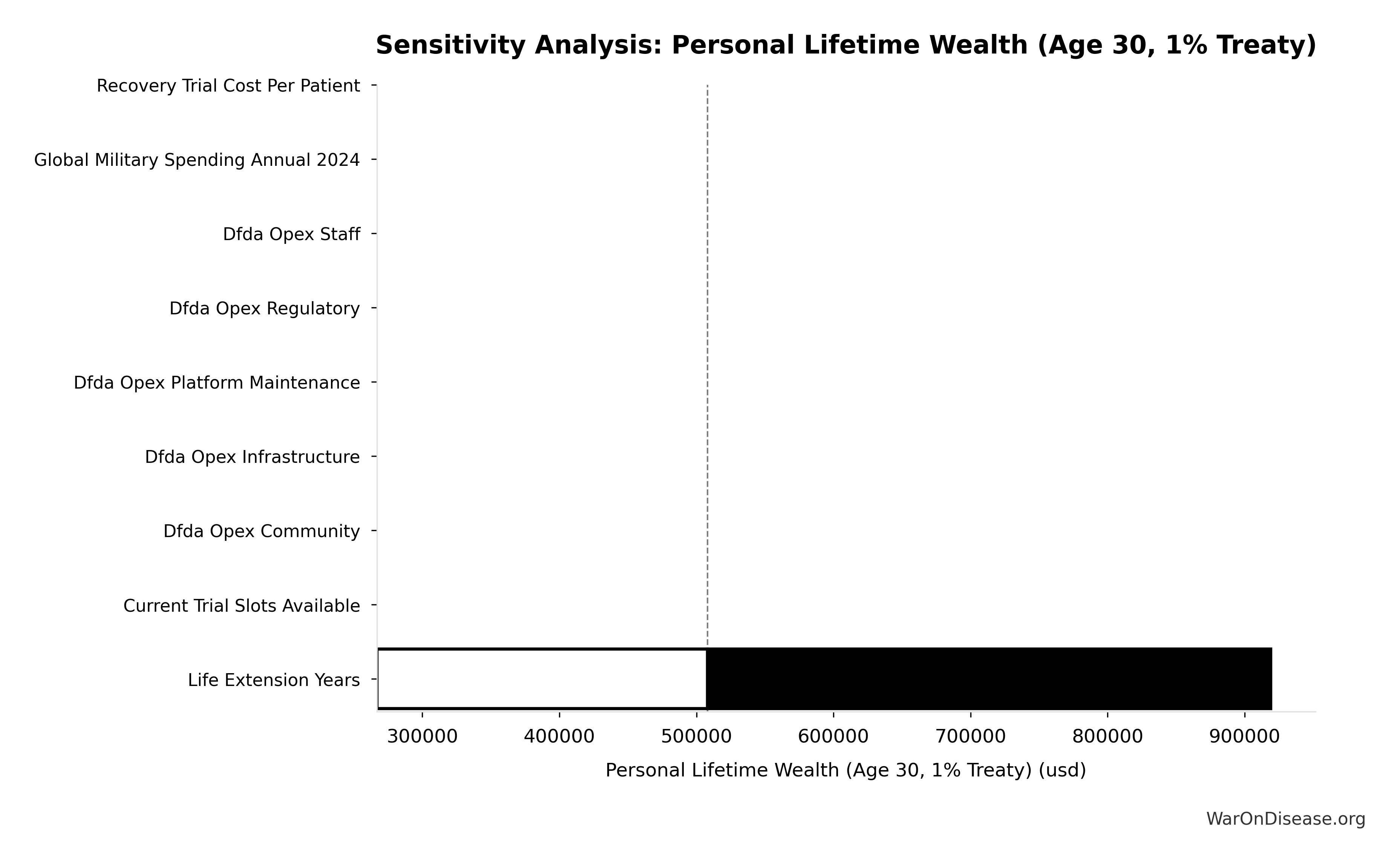
Simulation Results Summary: RECOVERY Trial Total QALYs Generated
| Statistic | Value |
|---|---|
| Baseline (deterministic) | 5 million |
| Mean (expected value) | 5.57 million |
| Median (50th percentile) | 4.36 million |
| Standard Deviation | 4.03 million |
| 90% Range (5th-95th percentile) | [1.51 million, 14.3 million] |
The histogram shows the distribution of RECOVERY Trial Total QALYs Generated across 10,000 Monte Carlo simulations. The CDF (right) shows the probability of the outcome exceeding any given value, which is useful for risk assessment.
Exceedance Probability
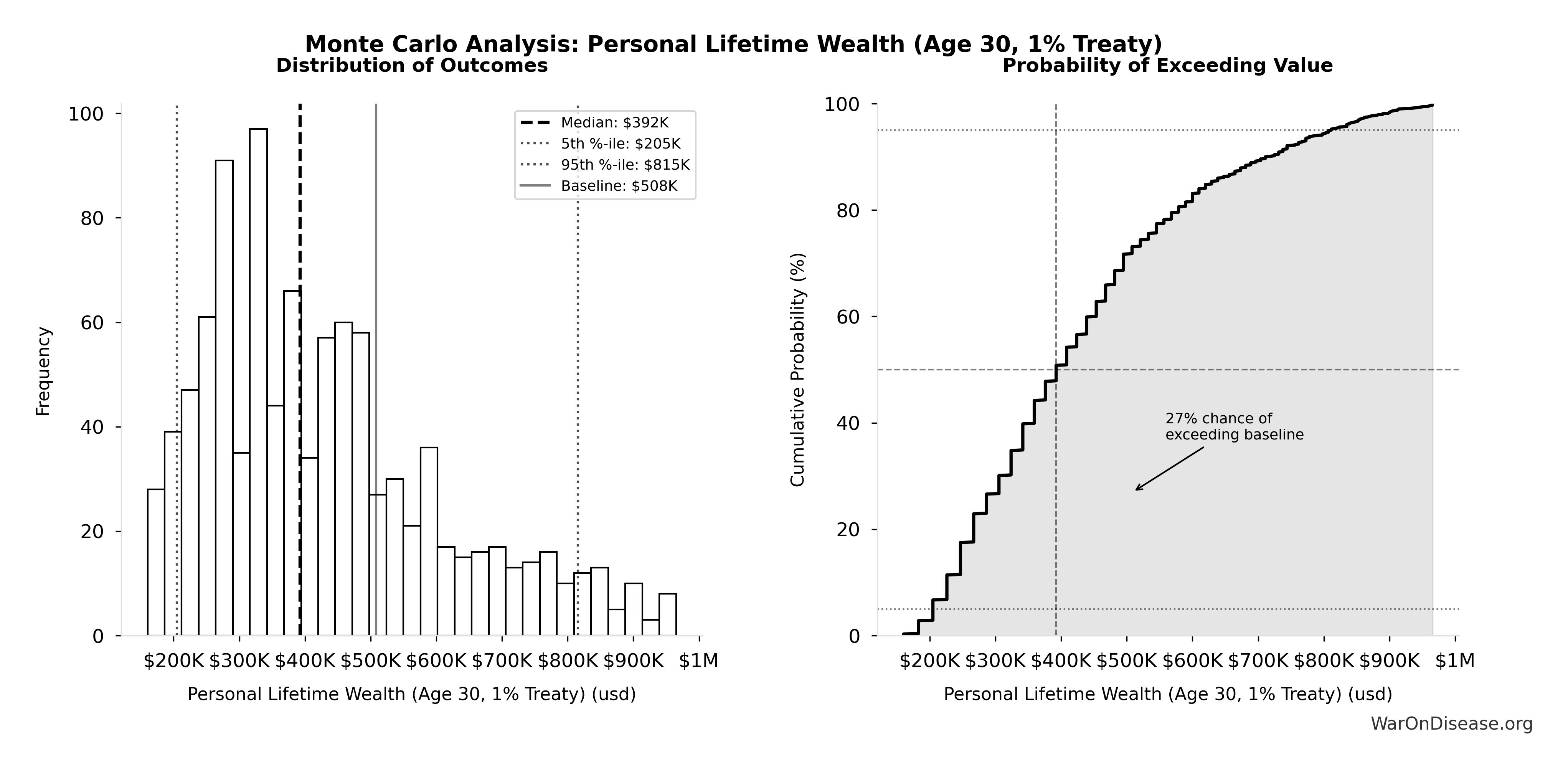
This exceedance probability chart shows the likelihood that RECOVERY Trial Total QALYs Generated will exceed any given threshold. Higher curves indicate more favorable outcomes with greater certainty.
Status Quo Average Years to First Treatment: 222 years
Note📊 Details
Average years until first treatment discovered for a typical disease under current system. At current discovery rates, the average disease waits half the total exploration time (~443/2 = ~222 years).
Inputs:
- Status Quo Therapeutic Space Exploration Time 🔢: 443 years
\[ \begin{gathered} T_{first,SQ} \\ = T_{queue,SQ} \times 0.5 \\ = 443 \times 0.5 \\ = 222 \end{gathered} \] where: \[ \begin{gathered} T_{queue,SQ} \\ = \frac{N_{untreated}}{Treatments_{new,ann}} \\ = \frac{6{,}650}{15} \\ = 443 \end{gathered} \] where: \[ \begin{gathered} N_{untreated} \\ = N_{rare} \times 0.95 \\ = 7{,}000 \times 0.95 \\ = 6{,}650 \end{gathered} \] Methodology:140
? Low confidence
Sensitivity Analysis
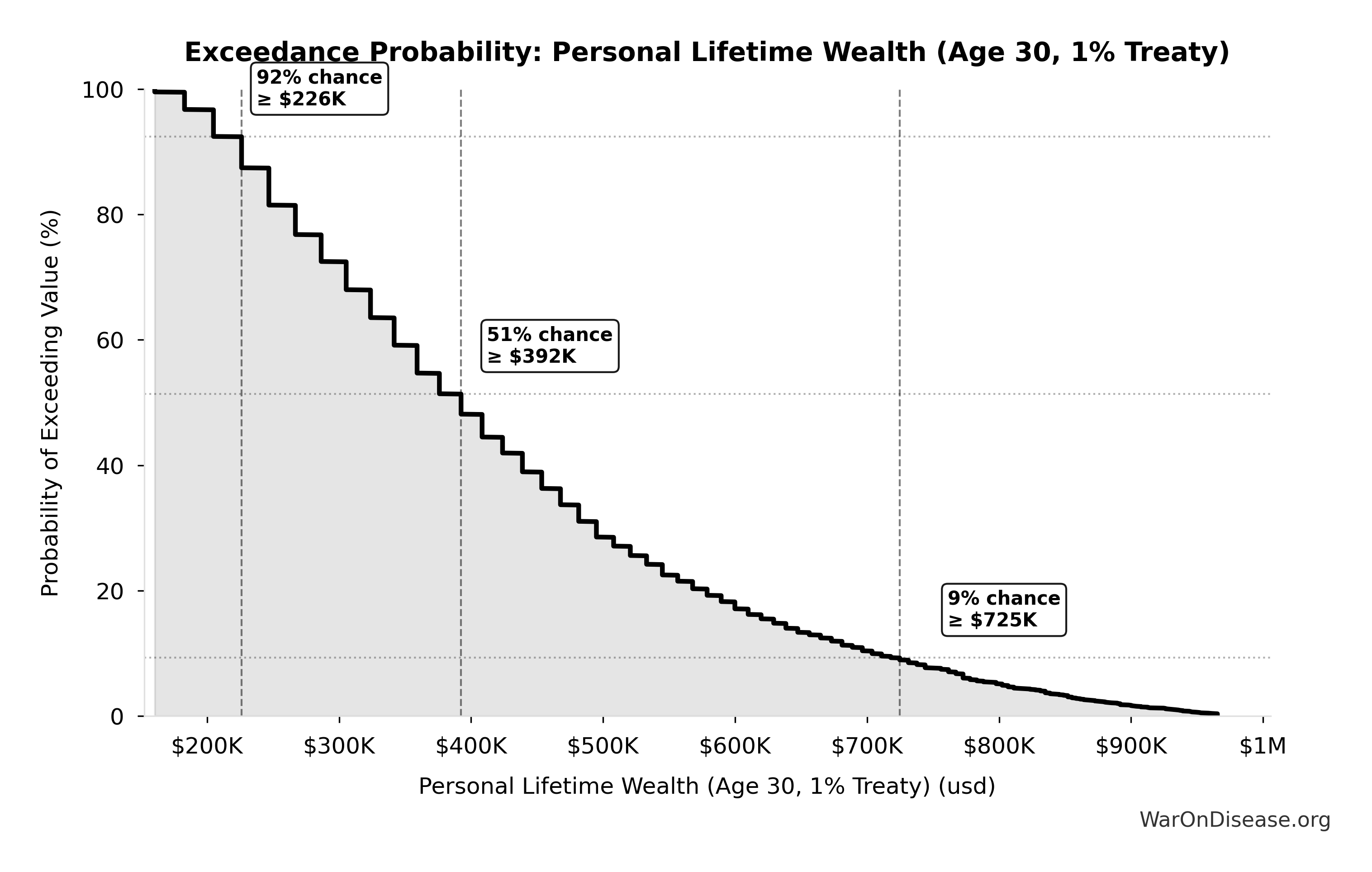
Sensitivity Indices for Status Quo Average Years to First Treatment
Regression-based sensitivity showing which inputs explain the most variance in the output.
| Input Parameter | Sensitivity Coefficient | Interpretation |
|---|---|---|
| Status Quo Therapeutic Space Exploration Time (years) | 1.0000 | Strong driver |
Interpretation: Standardized coefficients show the change in output (in SD units) per 1 SD change in input. Values near ±1 indicate strong influence; values exceeding ±1 may occur with correlated inputs.
Monte Carlo Distribution
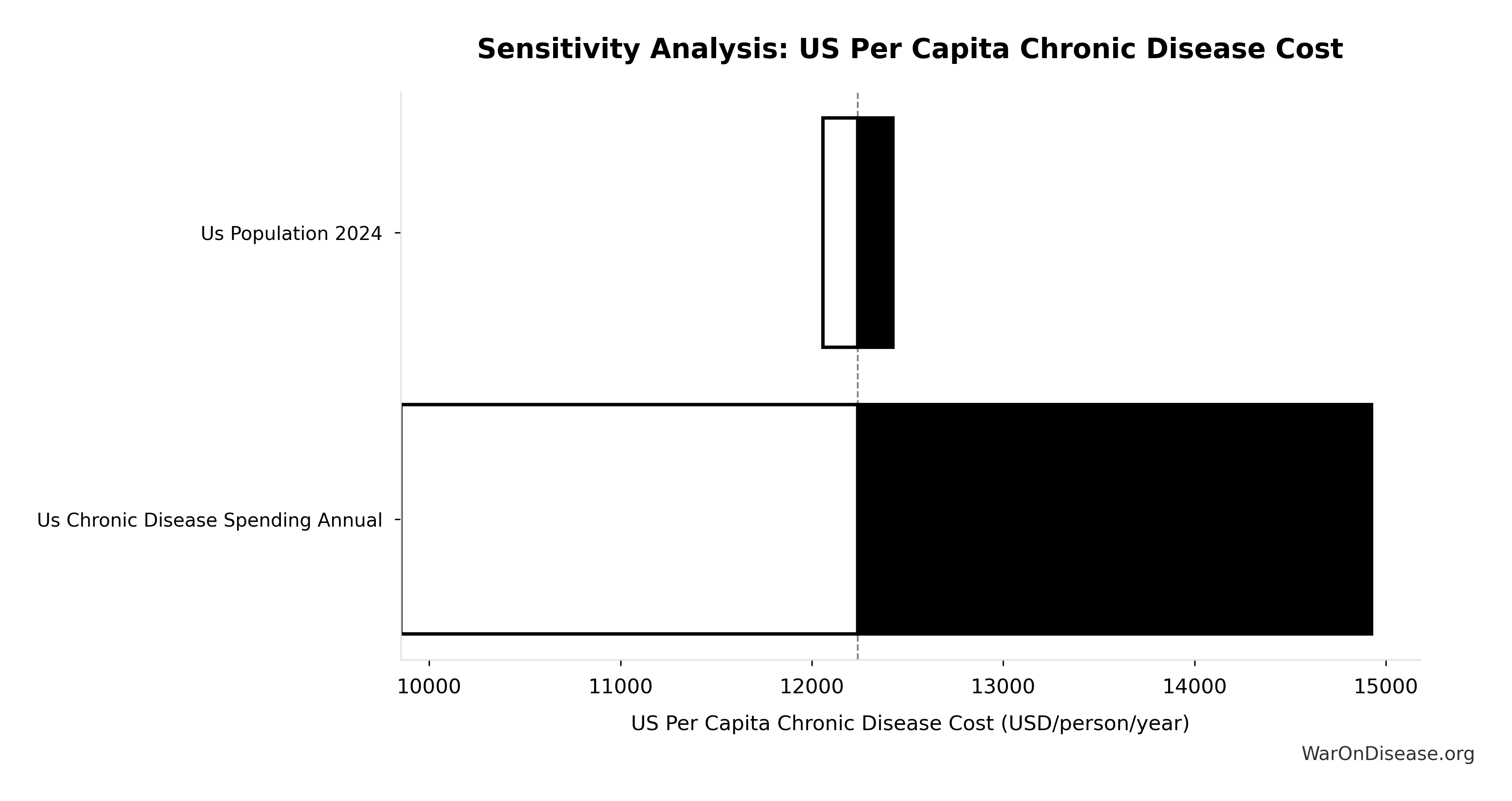
Simulation Results Summary: Status Quo Average Years to First Treatment
| Statistic | Value |
|---|---|
| Baseline (deterministic) | 222 |
| Mean (expected value) | 242 |
| Median (50th percentile) | 237 |
| Standard Deviation | 53.2 |
| 90% Range (5th-95th percentile) | [162, 356] |
The histogram shows the distribution of Status Quo Average Years to First Treatment across 10,000 Monte Carlo simulations. The CDF (right) shows the probability of the outcome exceeding any given value, which is useful for risk assessment.
Exceedance Probability
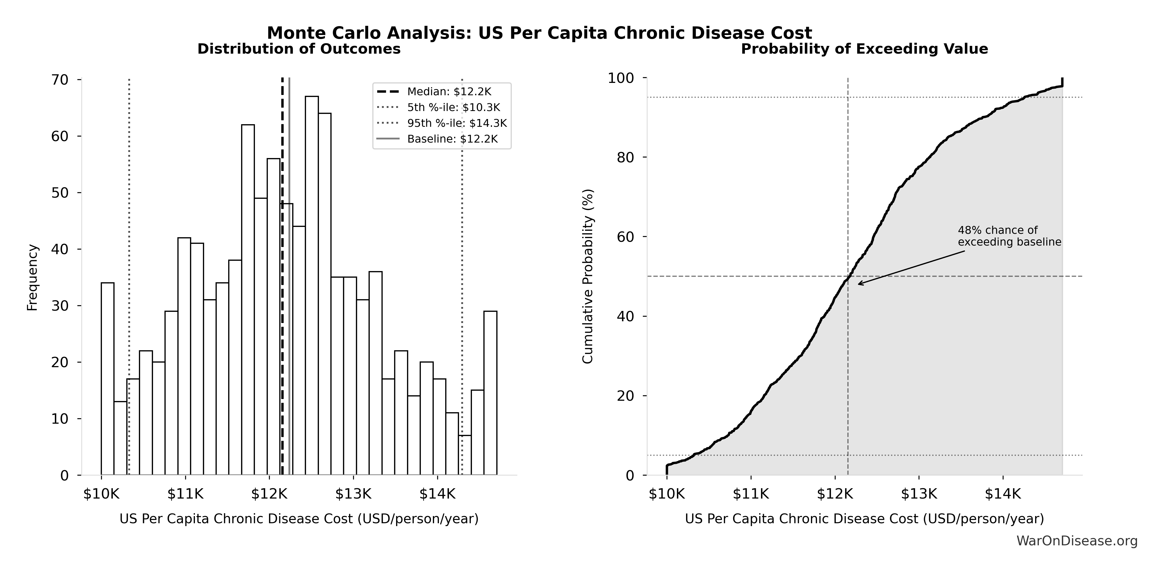
This exceedance probability chart shows the likelihood that Status Quo Average Years to First Treatment will exceed any given threshold. Higher curves indicate more favorable outcomes with greater certainty.
Status Quo Therapeutic Space Exploration Time: 443 years
Note📊 Details
Years to explore the entire therapeutic search space under current system. At current discovery rate of ~15 diseases/year getting first treatments, finding treatments for all ~6,650 untreated diseases would take ~443 years.
Inputs:
- Diseases Without Effective Treatment 🔢: 6.65 thousand diseases
- Diseases Getting First Treatment Per Year 📊: 15 diseases/year (95% CI: 8 diseases/year - 30 diseases/year)
\[ \begin{gathered} T_{queue,SQ} \\ = \frac{N_{untreated}}{Treatments_{new,ann}} \\ = \frac{6{,}650}{15} \\ = 443 \end{gathered} \] where: \[ \begin{gathered} N_{untreated} \\ = N_{rare} \times 0.95 \\ = 7{,}000 \times 0.95 \\ = 6{,}650 \end{gathered} \] Methodology:140
? Low confidence
Sensitivity Analysis
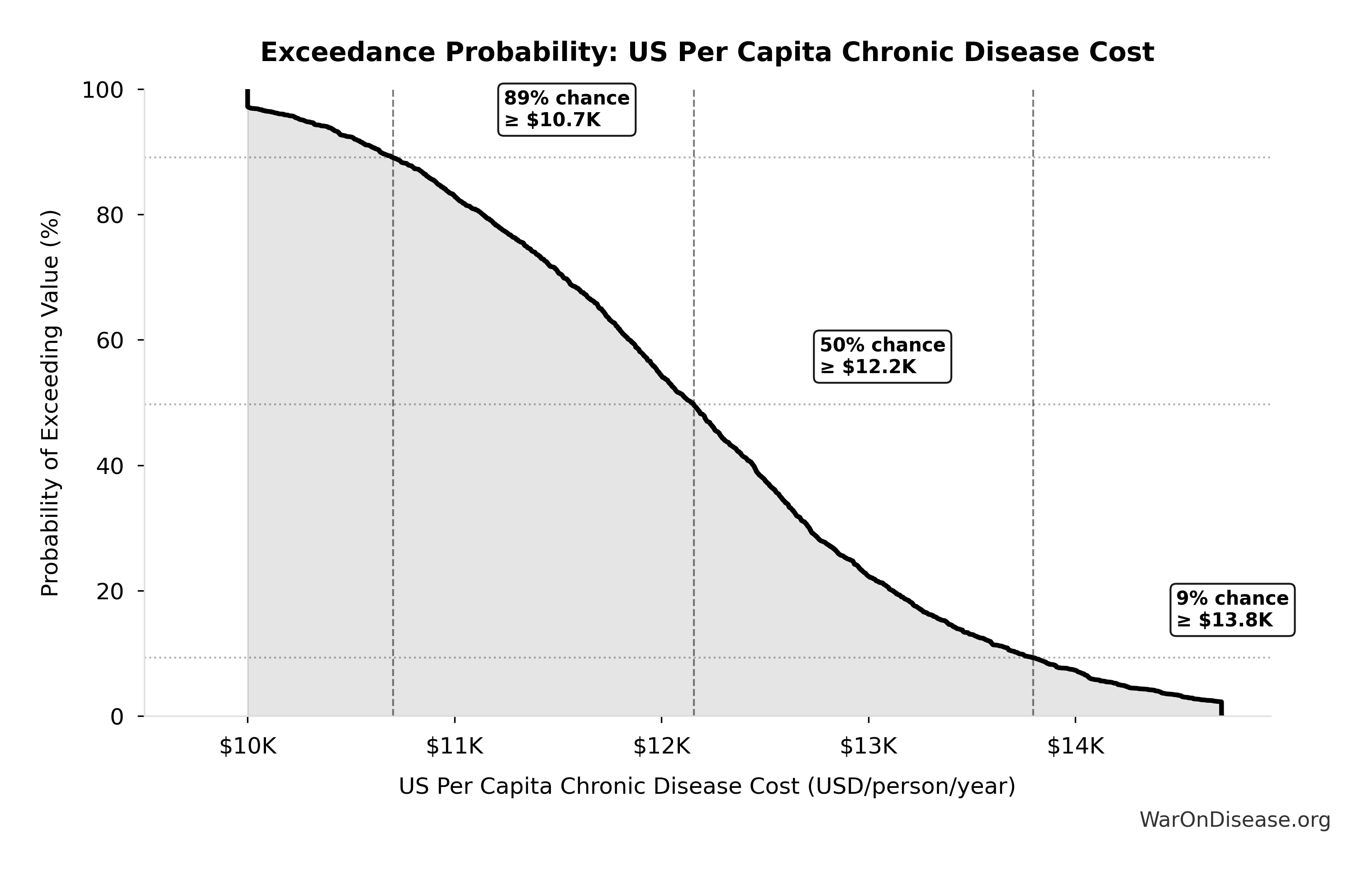
Sensitivity Indices for Status Quo Therapeutic Space Exploration Time
Regression-based sensitivity showing which inputs explain the most variance in the output.
| Input Parameter | Sensitivity Coefficient | Interpretation |
|---|---|---|
| Diseases Without Effective Treatment (diseases) | -0.7011 | Strong driver |
| Diseases Getting First Treatment Per Year (diseases/year) | -0.2360 | Weak driver |
Interpretation: Standardized coefficients show the change in output (in SD units) per 1 SD change in input. Values near ±1 indicate strong influence; values exceeding ±1 may occur with correlated inputs.
Monte Carlo Distribution
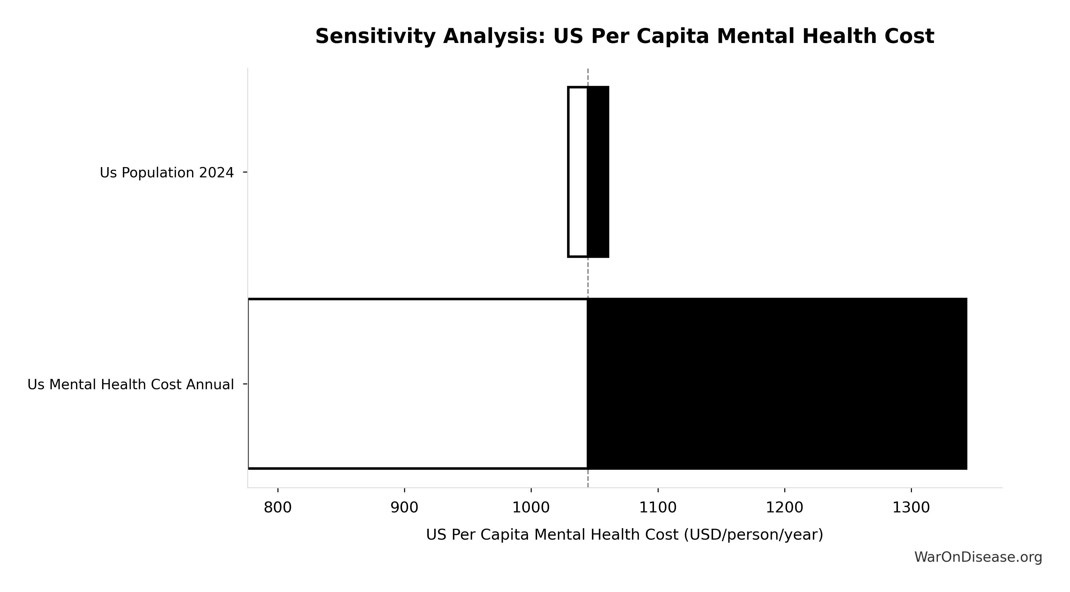
Simulation Results Summary: Status Quo Therapeutic Space Exploration Time
| Statistic | Value |
|---|---|
| Baseline (deterministic) | 443 |
| Mean (expected value) | 485 |
| Median (50th percentile) | 475 |
| Standard Deviation | 106 |
| 90% Range (5th-95th percentile) | [324, 712] |
The histogram shows the distribution of Status Quo Therapeutic Space Exploration Time across 10,000 Monte Carlo simulations. The CDF (right) shows the probability of the outcome exceeding any given value, which is useful for risk assessment.
Exceedance Probability
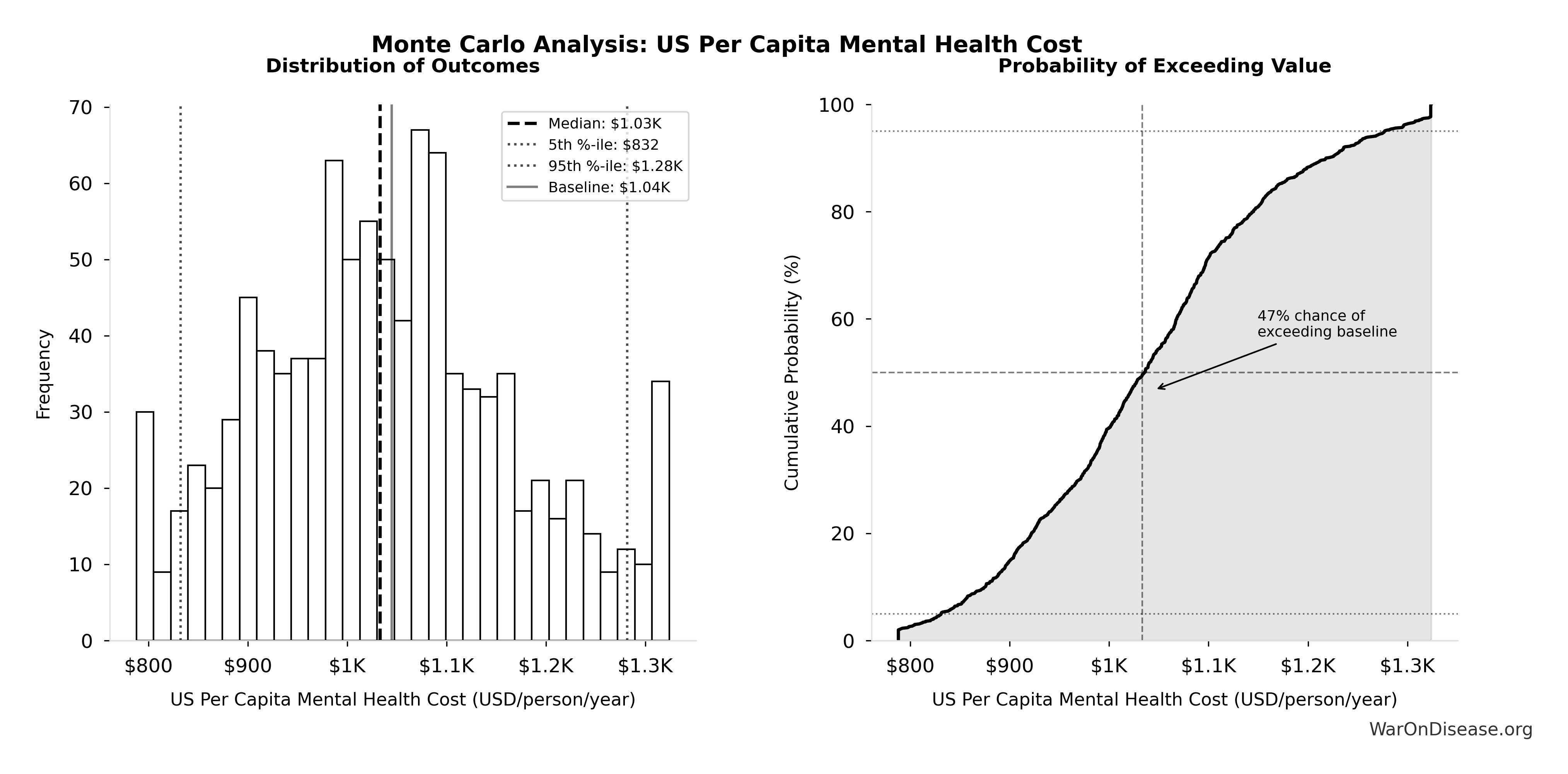
This exceedance probability chart shows the likelihood that Status Quo Therapeutic Space Exploration Time will exceed any given threshold. Higher curves indicate more favorable outcomes with greater certainty.
Thalidomide DALYs Per Event: 41.8 thousand DALYs
Note📊 Details
Total DALYs per US-scale thalidomide event (YLL + YLD)
Inputs:
- Thalidomide YLD Per Event 🔢: 13 thousand years
- Thalidomide YLL Per Event 🔢: 28.8 thousand years
\[ \begin{gathered} DALY_{thal} \\ = YLD_{thal} + YLL_{thal} \\ = 13{,}000 + 28{,}800 \\ = 41{,}800 \end{gathered} \] where: \[ \begin{gathered} YLD_{thal} \\ = DW_{thal} \times N_{thal,survive} \times LE_{thal} \\ = 0.4 \times 540 \times 60 \\ = 13{,}000 \end{gathered} \] where: \[ \begin{gathered} N_{thal,survive} \\ = N_{thal,US,prevent} \times (1 - Rate_{thal,mort}) \\ = 900 \times (1 - 40\%) \\ = 540 \end{gathered} \] where: \[ \begin{gathered} N_{thal,US,prevent} \\ = N_{thal,global} \times Pct_{US,1960} \\ = 15{,}000 \times 6\% \\ = 900 \end{gathered} \] where: \[ \begin{gathered} YLL_{thal} \\ = Deaths_{thal} \times 80 \\ = 360 \times 80 \\ = 28{,}800 \end{gathered} \] where: \[ \begin{gathered} Deaths_{thal} \\ = Rate_{thal,mort} \times N_{thal,US,prevent} \\ = 40\% \times 900 \\ = 360 \end{gathered} \] ~ Medium confidence
Sensitivity Analysis
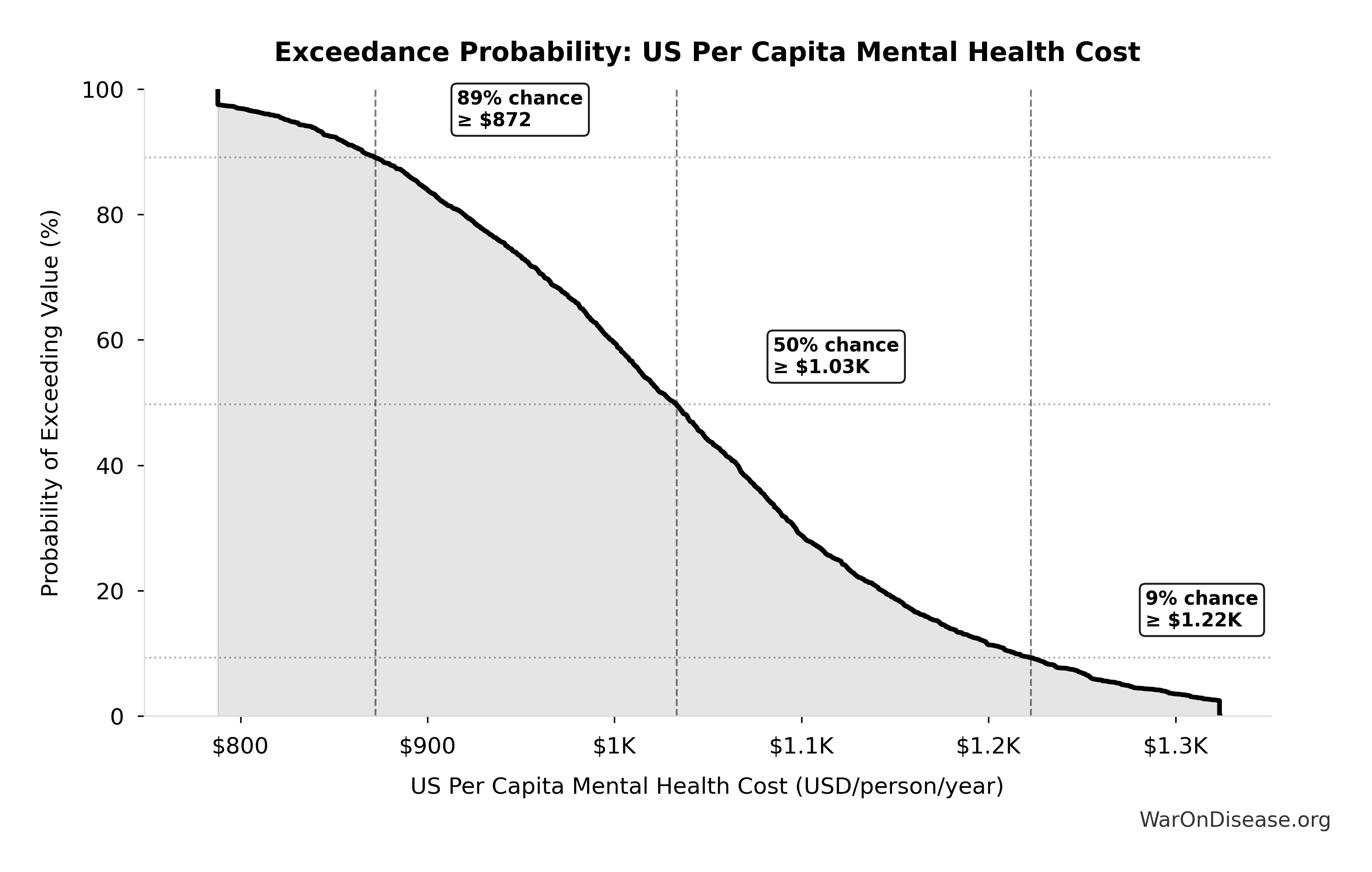
Sensitivity Indices for Thalidomide DALYs Per Event
Regression-based sensitivity showing which inputs explain the most variance in the output.
| Input Parameter | Sensitivity Coefficient | Interpretation |
|---|---|---|
| Thalidomide YLL Per Event (years) | 0.6300 | Strong driver |
| Thalidomide YLD Per Event (years) | 0.3701 | Moderate driver |
Interpretation: Standardized coefficients show the change in output (in SD units) per 1 SD change in input. Values near ±1 indicate strong influence; values exceeding ±1 may occur with correlated inputs.
Monte Carlo Distribution
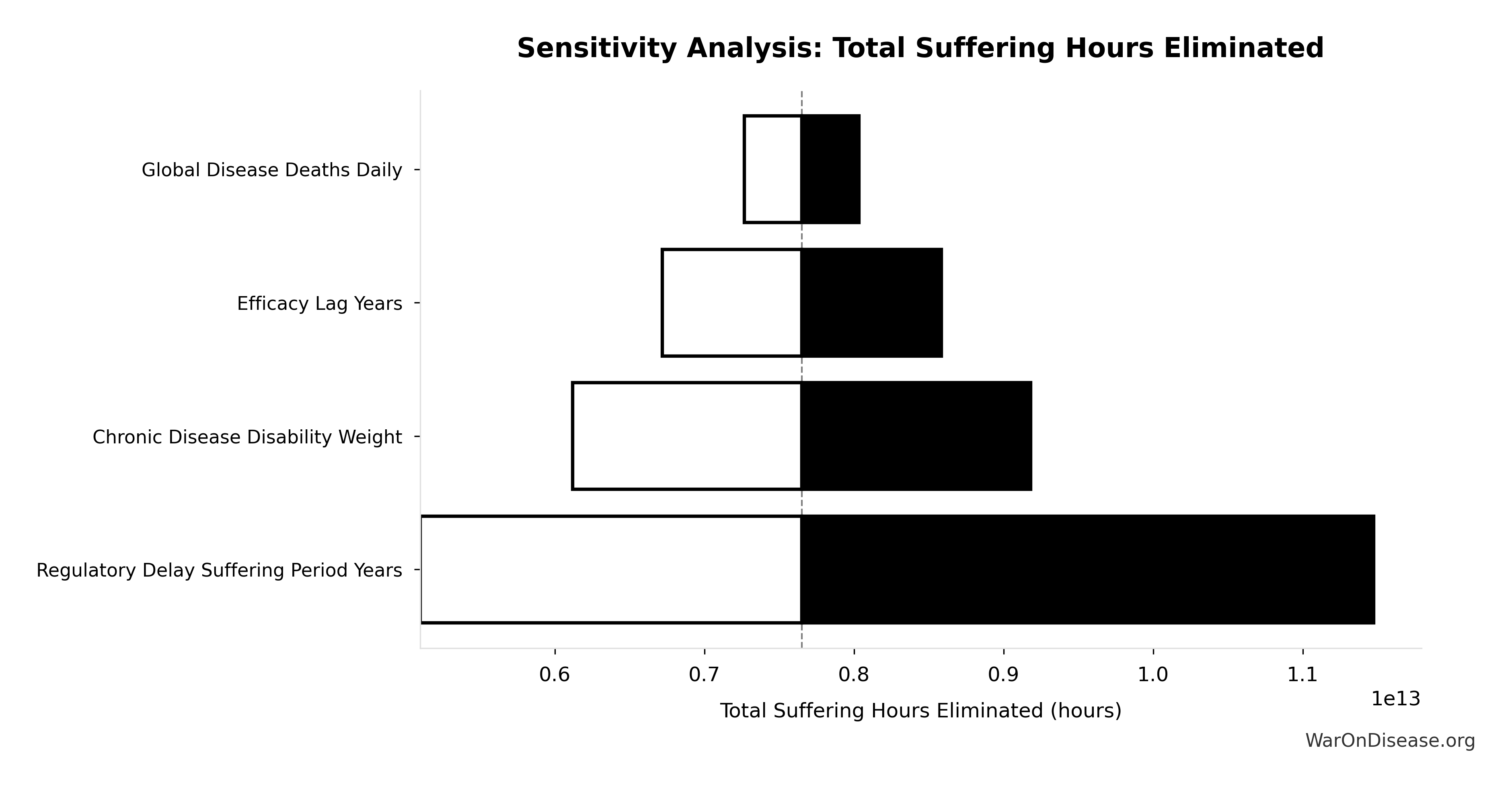
Simulation Results Summary: Thalidomide DALYs Per Event
| Statistic | Value |
|---|---|
| Baseline (deterministic) | 41.8 thousand |
| Mean (expected value) | 42.5 thousand |
| Median (50th percentile) | 40.8 thousand |
| Standard Deviation | 12.2 thousand |
| 90% Range (5th-95th percentile) | [24.8 thousand, 67.1 thousand] |
The histogram shows the distribution of Thalidomide DALYs Per Event across 10,000 Monte Carlo simulations. The CDF (right) shows the probability of the outcome exceeding any given value, which is useful for risk assessment.
Exceedance Probability
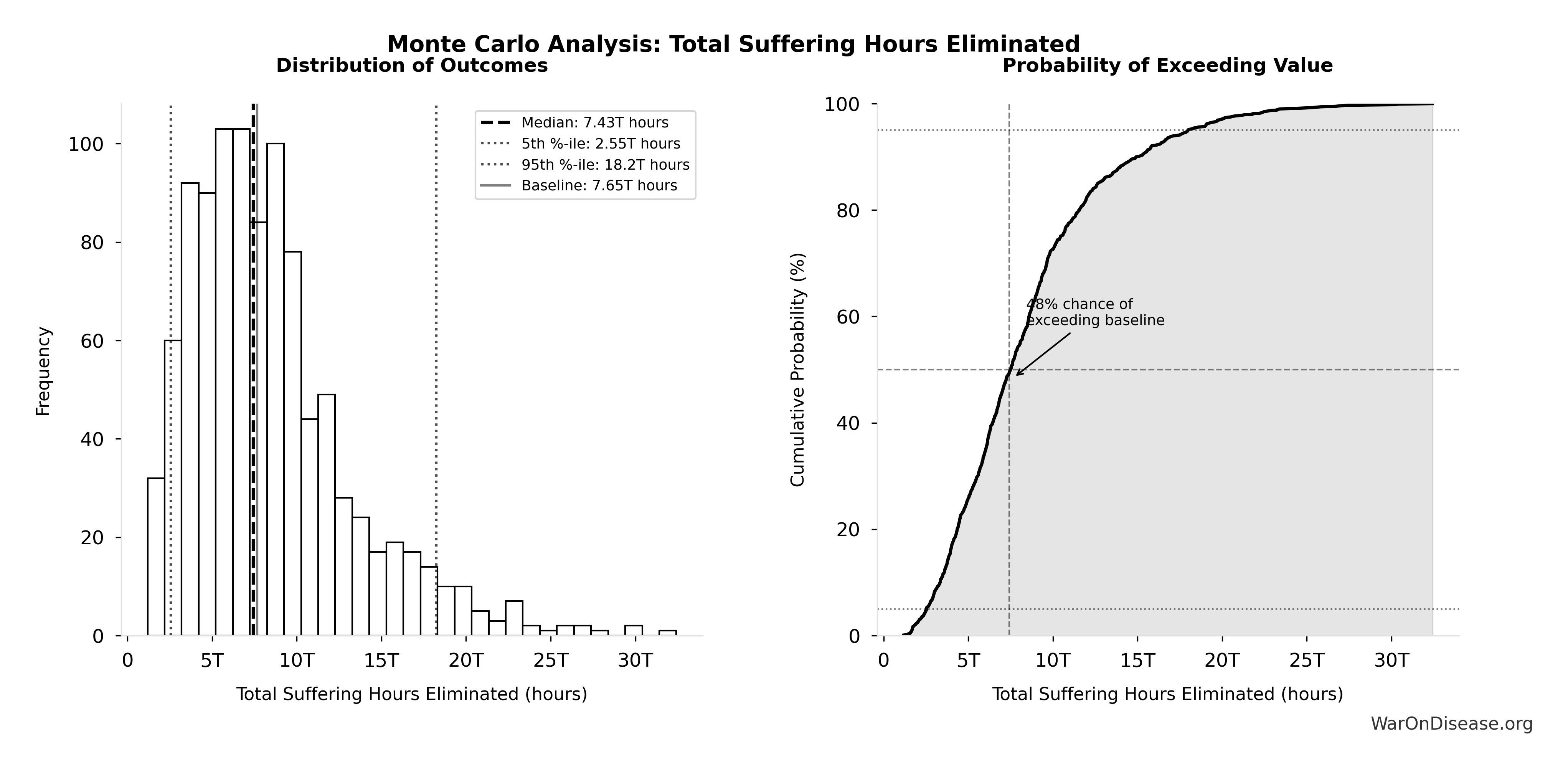
This exceedance probability chart shows the likelihood that Thalidomide DALYs Per Event will exceed any given threshold. Higher curves indicate more favorable outcomes with greater certainty.
Thalidomide Deaths Per Event: 360 deaths
Note📊 Details
Deaths per US-scale thalidomide event
Inputs:
- Thalidomide Mortality Rate 📊: 40% (95% CI: 35% - 45%)
- Thalidomide US Cases Prevented 🔢: 900 cases
\[ \begin{gathered} Deaths_{thal} \\ = Rate_{thal,mort} \times N_{thal,US,prevent} \\ = 40\% \times 900 \\ = 360 \end{gathered} \] where: \[ \begin{gathered} N_{thal,US,prevent} \\ = N_{thal,global} \times Pct_{US,1960} \\ = 15{,}000 \times 6\% \\ = 900 \end{gathered} \] ~ Medium confidence
Sensitivity Analysis
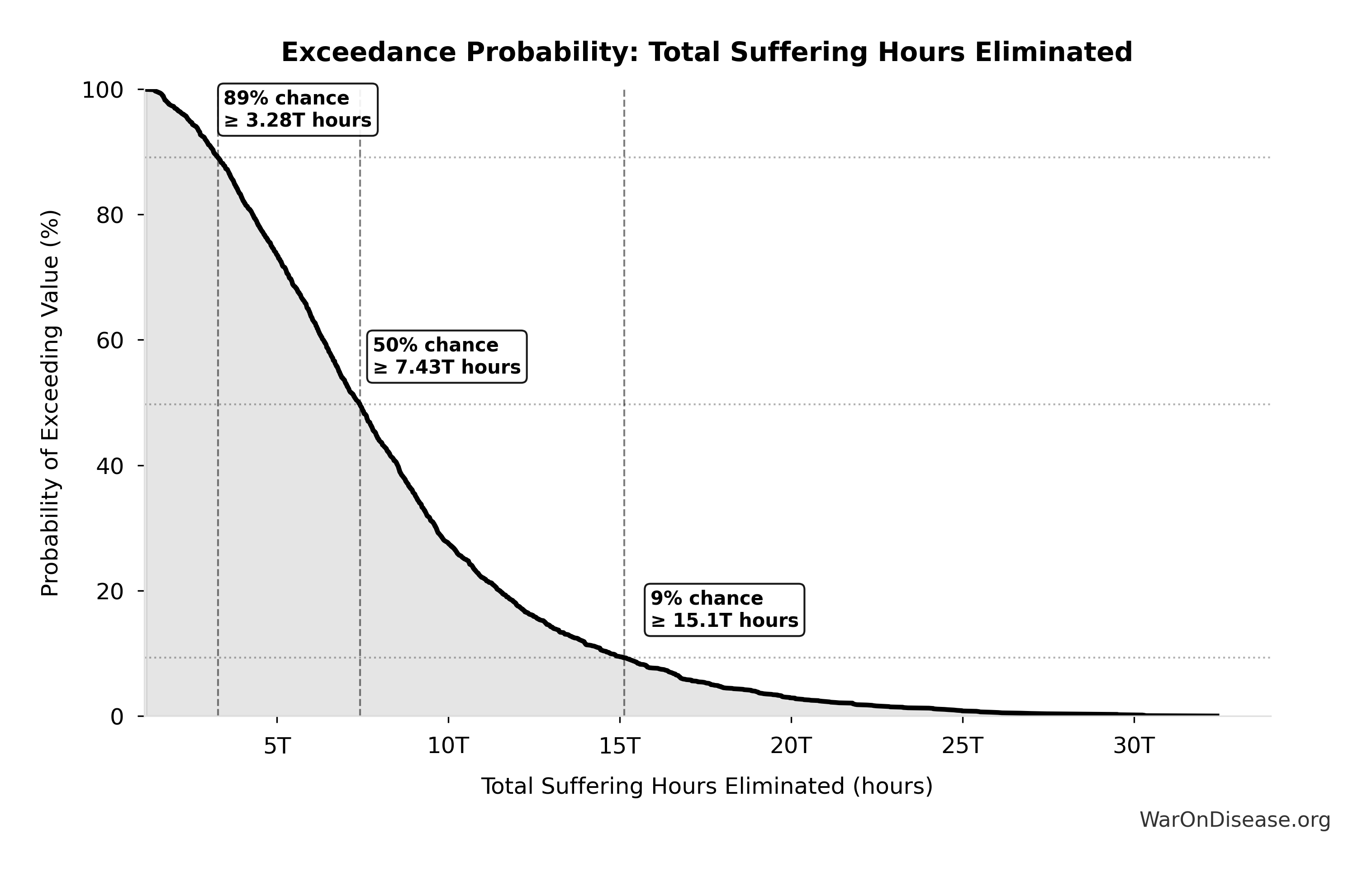
Sensitivity Indices for Thalidomide Deaths Per Event
Regression-based sensitivity showing which inputs explain the most variance in the output.
| Input Parameter | Sensitivity Coefficient | Interpretation |
|---|---|---|
| Thalidomide US Cases Prevented (cases) | 1.5027 | Strong driver |
| Thalidomide Mortality Rate (percentage) | -0.5048 | Strong driver |
Interpretation: Standardized coefficients show the change in output (in SD units) per 1 SD change in input. Values near ±1 indicate strong influence; values exceeding ±1 may occur with correlated inputs.
Monte Carlo Distribution
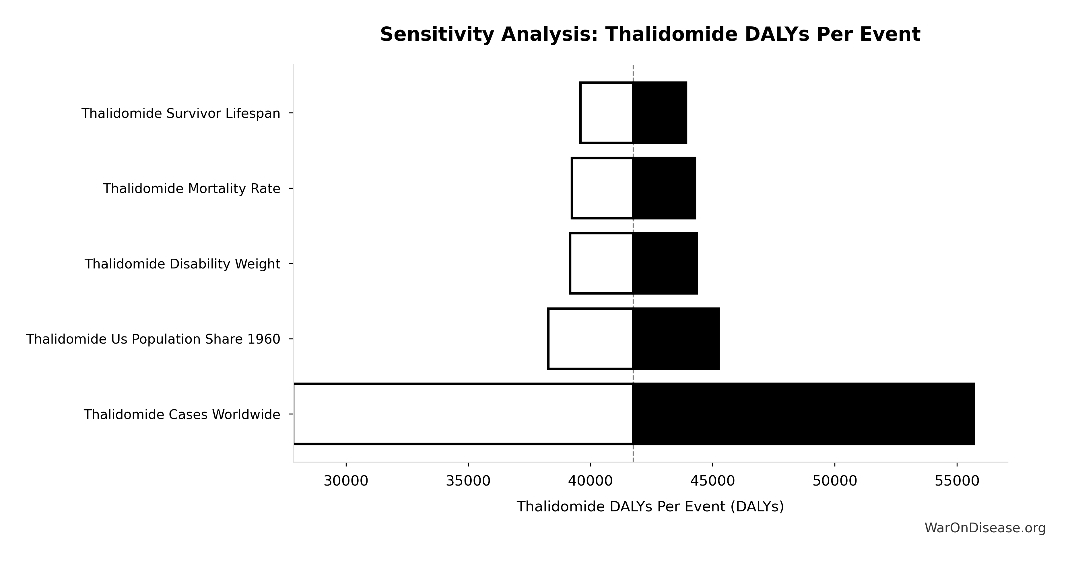
Simulation Results Summary: Thalidomide Deaths Per Event
| Statistic | Value |
|---|---|
| Baseline (deterministic) | 360 |
| Mean (expected value) | 364 |
| Median (50th percentile) | 353 |
| Standard Deviation | 95.8 |
| 90% Range (5th-95th percentile) | [223, 556] |
The histogram shows the distribution of Thalidomide Deaths Per Event across 10,000 Monte Carlo simulations. The CDF (right) shows the probability of the outcome exceeding any given value, which is useful for risk assessment.
Exceedance Probability
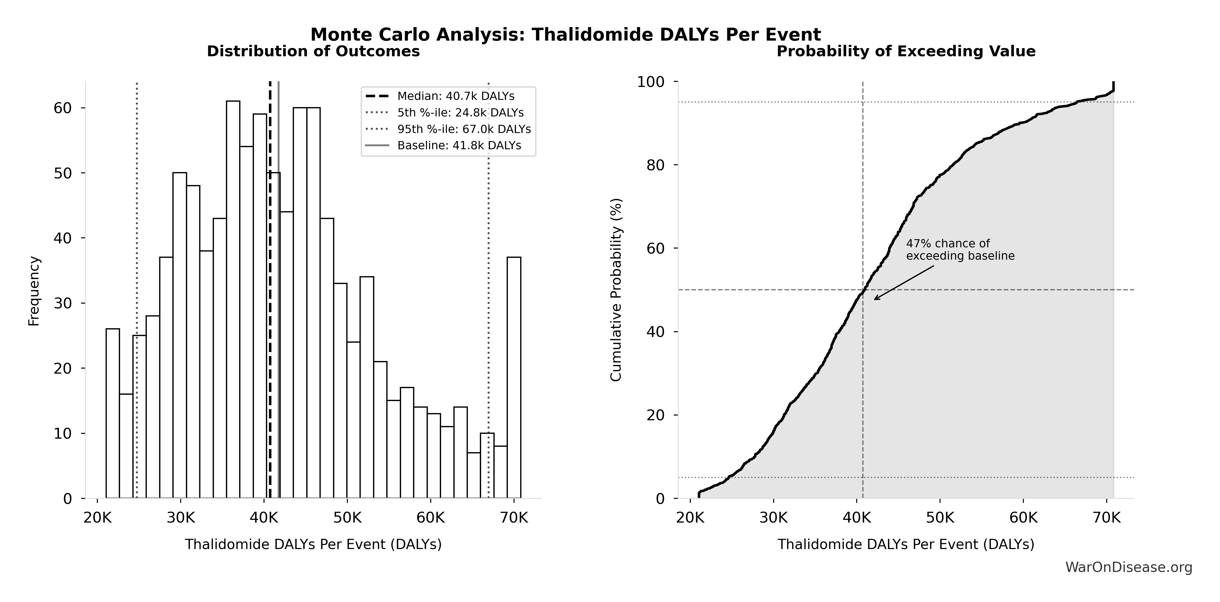
This exceedance probability chart shows the likelihood that Thalidomide Deaths Per Event will exceed any given threshold. Higher curves indicate more favorable outcomes with greater certainty.
Thalidomide Survivors Per Event: 540 cases
Note📊 Details
Survivors per US-scale thalidomide event
Inputs:
- Thalidomide Mortality Rate 📊: 40% (95% CI: 35% - 45%)
- Thalidomide US Cases Prevented 🔢: 900 cases
\[ \begin{gathered} N_{thal,survive} \\ = N_{thal,US,prevent} \times (1 - Rate_{thal,mort}) \\ = 900 \times (1 - 40\%) \\ = 540 \end{gathered} \] where: \[ \begin{gathered} N_{thal,US,prevent} \\ = N_{thal,global} \times Pct_{US,1960} \\ = 15{,}000 \times 6\% \\ = 900 \end{gathered} \] ~ Medium confidence
Sensitivity Analysis
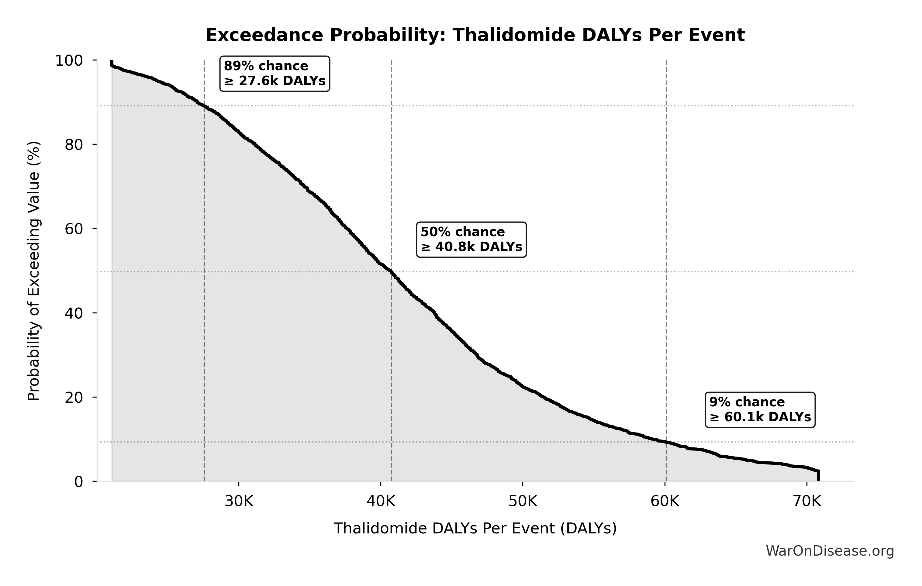
Sensitivity Indices for Thalidomide Survivors Per Event
Regression-based sensitivity showing which inputs explain the most variance in the output.
| Input Parameter | Sensitivity Coefficient | Interpretation |
|---|---|---|
| Thalidomide Mortality Rate (percentage) | 0.5607 | Strong driver |
| Thalidomide US Cases Prevented (cases) | 0.4398 | Moderate driver |
Interpretation: Standardized coefficients show the change in output (in SD units) per 1 SD change in input. Values near ±1 indicate strong influence; values exceeding ±1 may occur with correlated inputs.
Monte Carlo Distribution

Simulation Results Summary: Thalidomide Survivors Per Event
| Statistic | Value |
|---|---|
| Baseline (deterministic) | 540 |
| Mean (expected value) | 537 |
| Median (50th percentile) | 531 |
| Standard Deviation | 86.3 |
| 90% Range (5th-95th percentile) | [399, 698] |
The histogram shows the distribution of Thalidomide Survivors Per Event across 10,000 Monte Carlo simulations. The CDF (right) shows the probability of the outcome exceeding any given value, which is useful for risk assessment.
Exceedance Probability
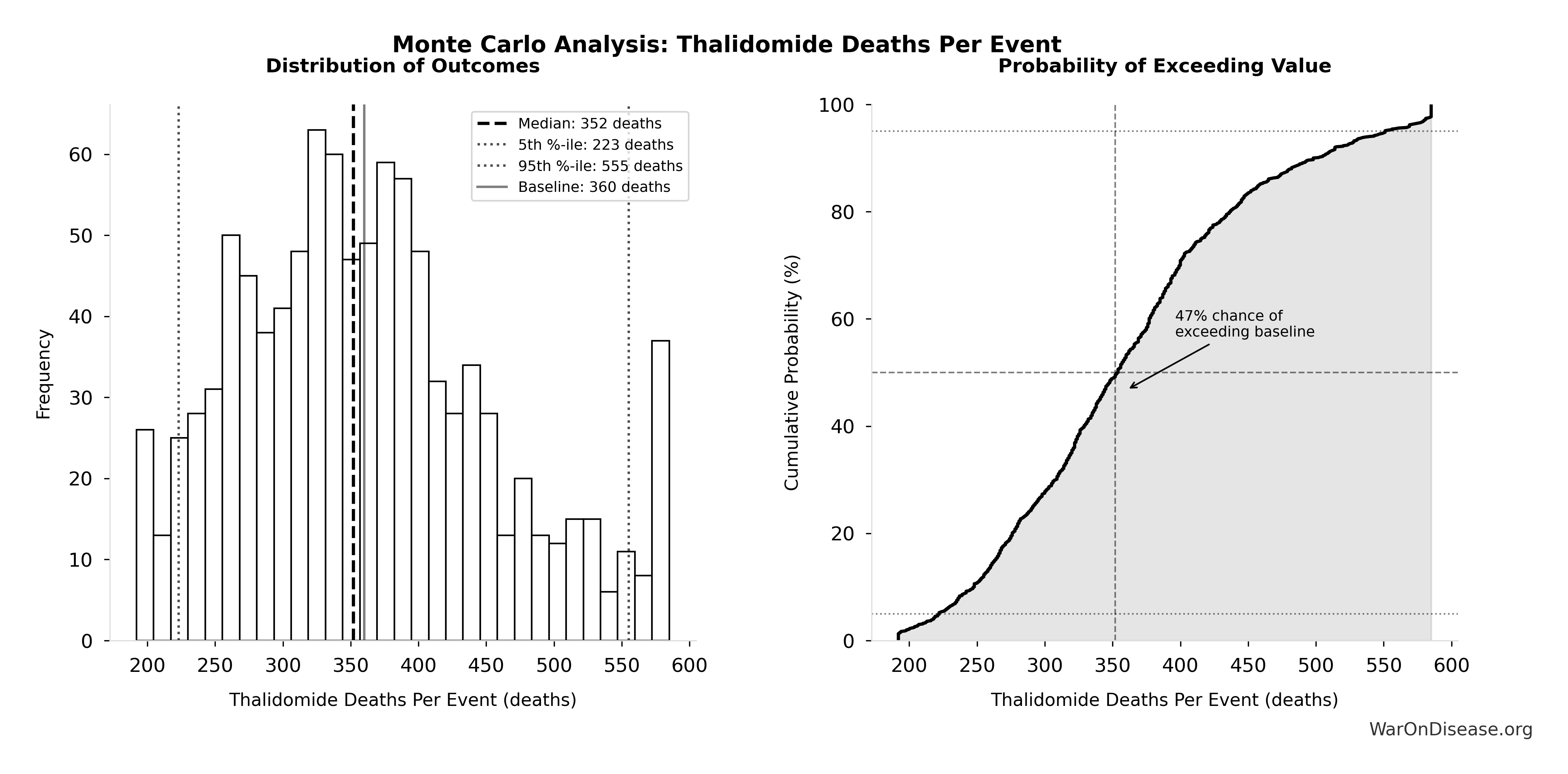
This exceedance probability chart shows the likelihood that Thalidomide Survivors Per Event will exceed any given threshold. Higher curves indicate more favorable outcomes with greater certainty.
Thalidomide US Cases Prevented: 900 cases
Note📊 Details
Estimated US thalidomide cases prevented by FDA rejection
Inputs:
- Thalidomide Cases Worldwide 📊: 15 thousand cases (95% CI: 10 thousand cases - 20 thousand cases)
- US Population Share 1960 📊: 6% (95% CI: 5.5% - 6.5%)
\[ \begin{gathered} N_{thal,US,prevent} \\ = N_{thal,global} \times Pct_{US,1960} \\ = 15{,}000 \times 6\% \\ = 900 \end{gathered} \]
~ Medium confidence
Sensitivity Analysis
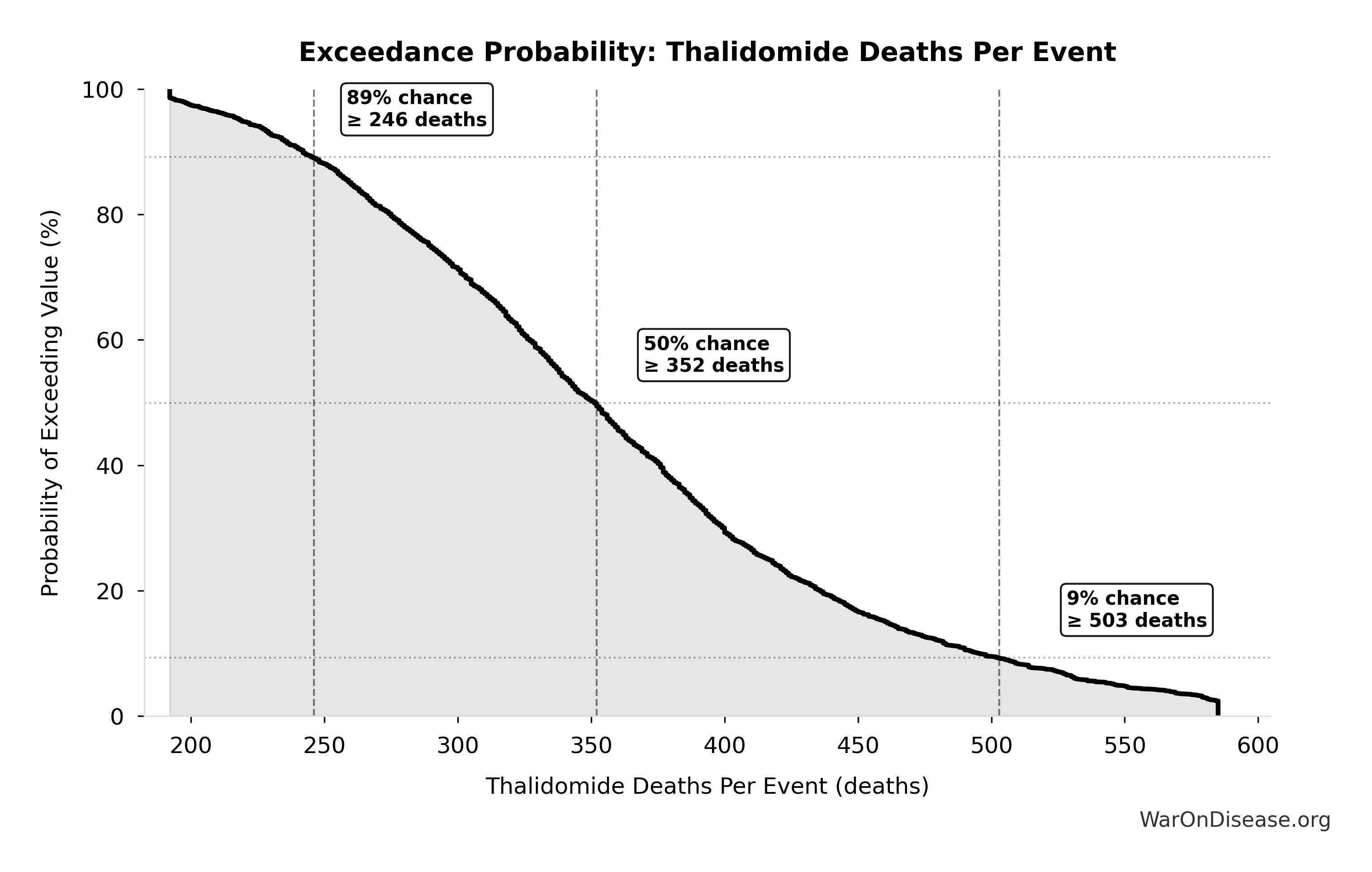
Sensitivity Indices for Thalidomide US Cases Prevented
Regression-based sensitivity showing which inputs explain the most variance in the output.
| Input Parameter | Sensitivity Coefficient | Interpretation |
|---|---|---|
| Thalidomide Cases Worldwide (cases) | 1.3746 | Strong driver |
| US Population Share 1960 (percentage) | -0.3756 | Moderate driver |
Interpretation: Standardized coefficients show the change in output (in SD units) per 1 SD change in input. Values near ±1 indicate strong influence; values exceeding ±1 may occur with correlated inputs.
Monte Carlo Distribution
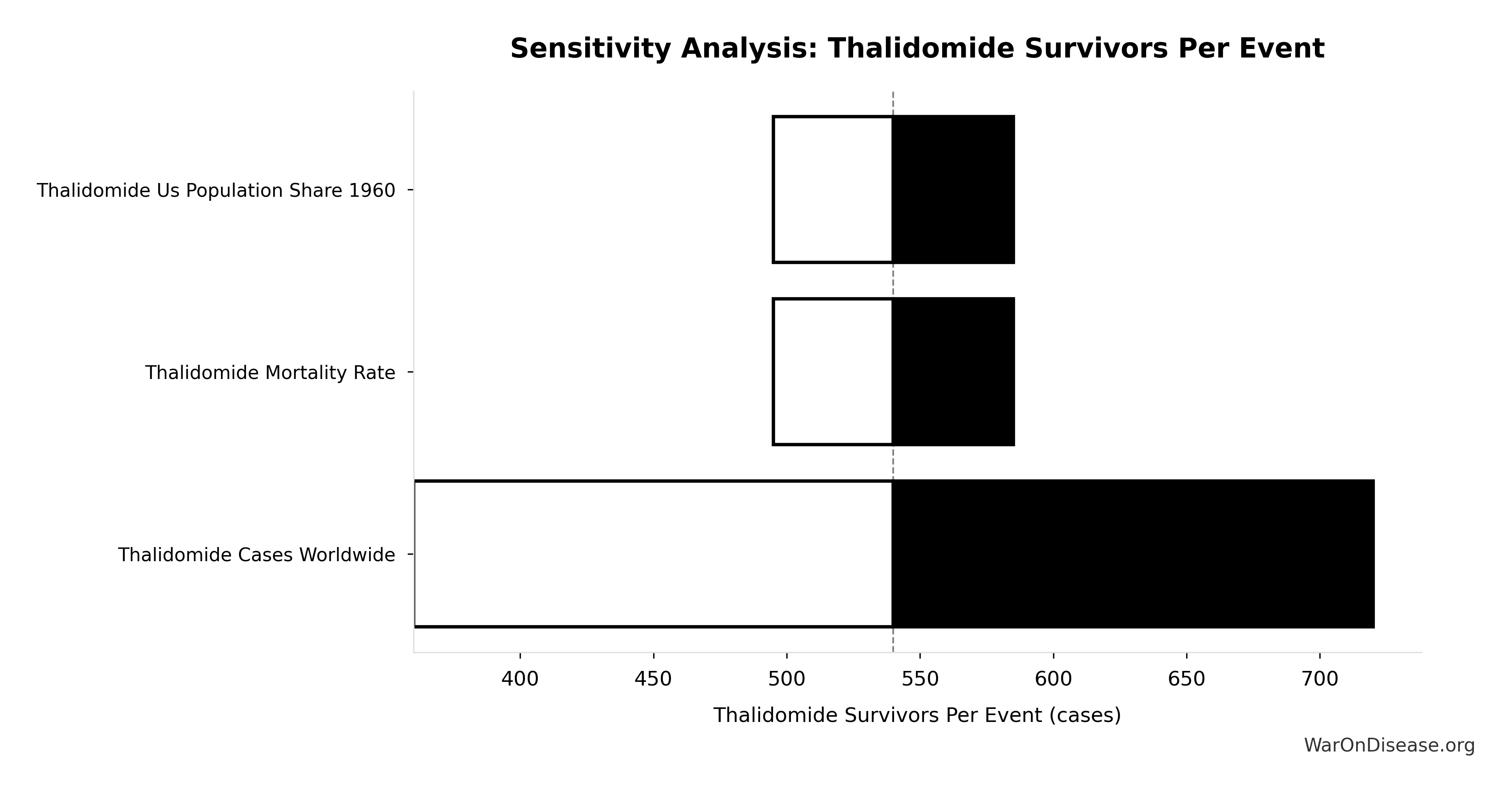
Simulation Results Summary: Thalidomide US Cases Prevented
| Statistic | Value |
|---|---|
| Baseline (deterministic) | 900 |
| Mean (expected value) | 901 |
| Median (50th percentile) | 884 |
| Standard Deviation | 182 |
| 90% Range (5th-95th percentile) | [622, 1.25 thousand] |
The histogram shows the distribution of Thalidomide US Cases Prevented across 10,000 Monte Carlo simulations. The CDF (right) shows the probability of the outcome exceeding any given value, which is useful for risk assessment.
Exceedance Probability
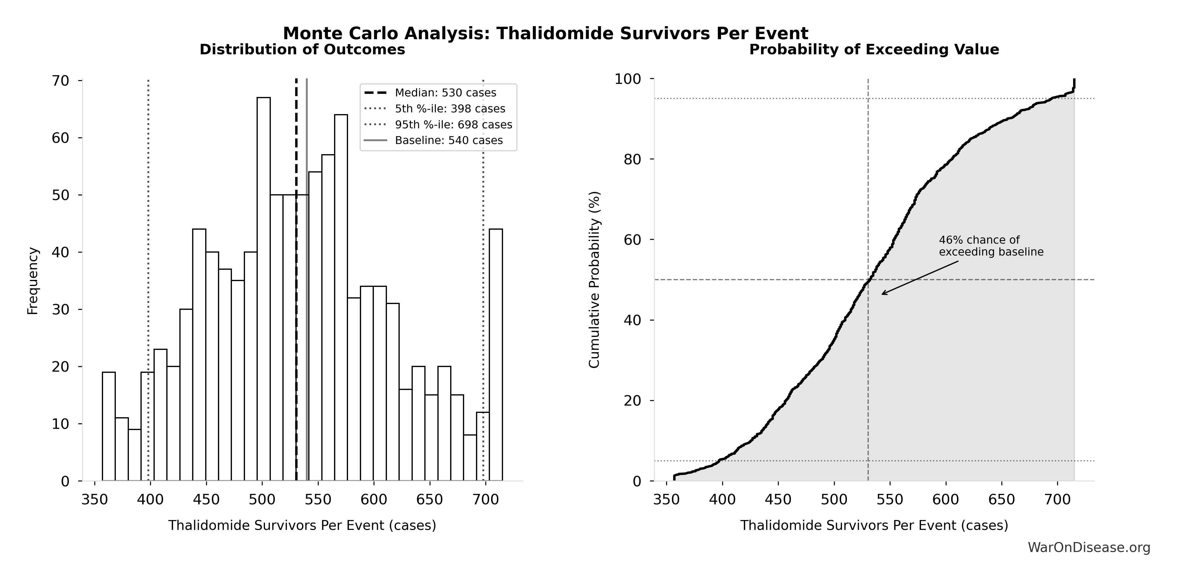
This exceedance probability chart shows the likelihood that Thalidomide US Cases Prevented will exceed any given threshold. Higher curves indicate more favorable outcomes with greater certainty.
Thalidomide YLD Per Event: 13 thousand years
Note📊 Details
Years Lived with Disability per thalidomide event
Inputs:
- Thalidomide Disability Weight 📊: 0.4:1 (95% CI: 0.32:1 - 0.48:1)
- Thalidomide Survivors Per Event 🔢: 540 cases
- Thalidomide Survivor Lifespan 📊: 60 years (95% CI: 50 years - 70 years)
\[ \begin{gathered} YLD_{thal} \\ = DW_{thal} \times N_{thal,survive} \times LE_{thal} \\ = 0.4 \times 540 \times 60 \\ = 13{,}000 \end{gathered} \] where: \[ \begin{gathered} N_{thal,survive} \\ = N_{thal,US,prevent} \times (1 - Rate_{thal,mort}) \\ = 900 \times (1 - 40\%) \\ = 540 \end{gathered} \] where: \[ \begin{gathered} N_{thal,US,prevent} \\ = N_{thal,global} \times Pct_{US,1960} \\ = 15{,}000 \times 6\% \\ = 900 \end{gathered} \] ~ Medium confidence
Sensitivity Analysis
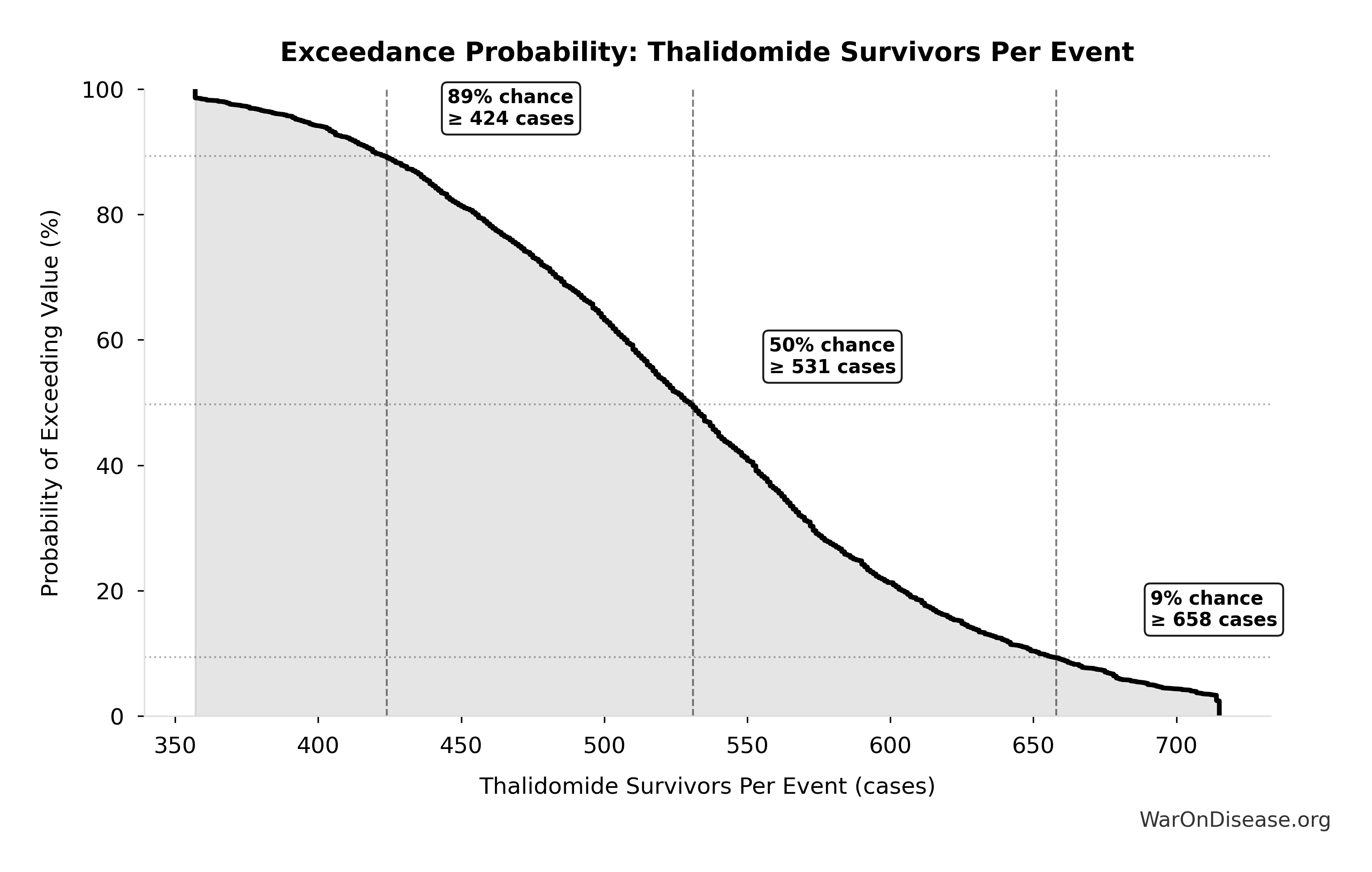
Sensitivity Indices for Thalidomide YLD Per Event
Regression-based sensitivity showing which inputs explain the most variance in the output.
| Input Parameter | Sensitivity Coefficient | Interpretation |
|---|---|---|
| Thalidomide Disability Weight (ratio) | 28.4785 | Strong driver |
| Thalidomide Survivor Lifespan (years) | -23.4440 | Strong driver |
| Thalidomide Survivors Per Event (cases) | -4.0444 | Strong driver |
Interpretation: Standardized coefficients show the change in output (in SD units) per 1 SD change in input. Values near ±1 indicate strong influence; values exceeding ±1 may occur with correlated inputs.
Monte Carlo Distribution
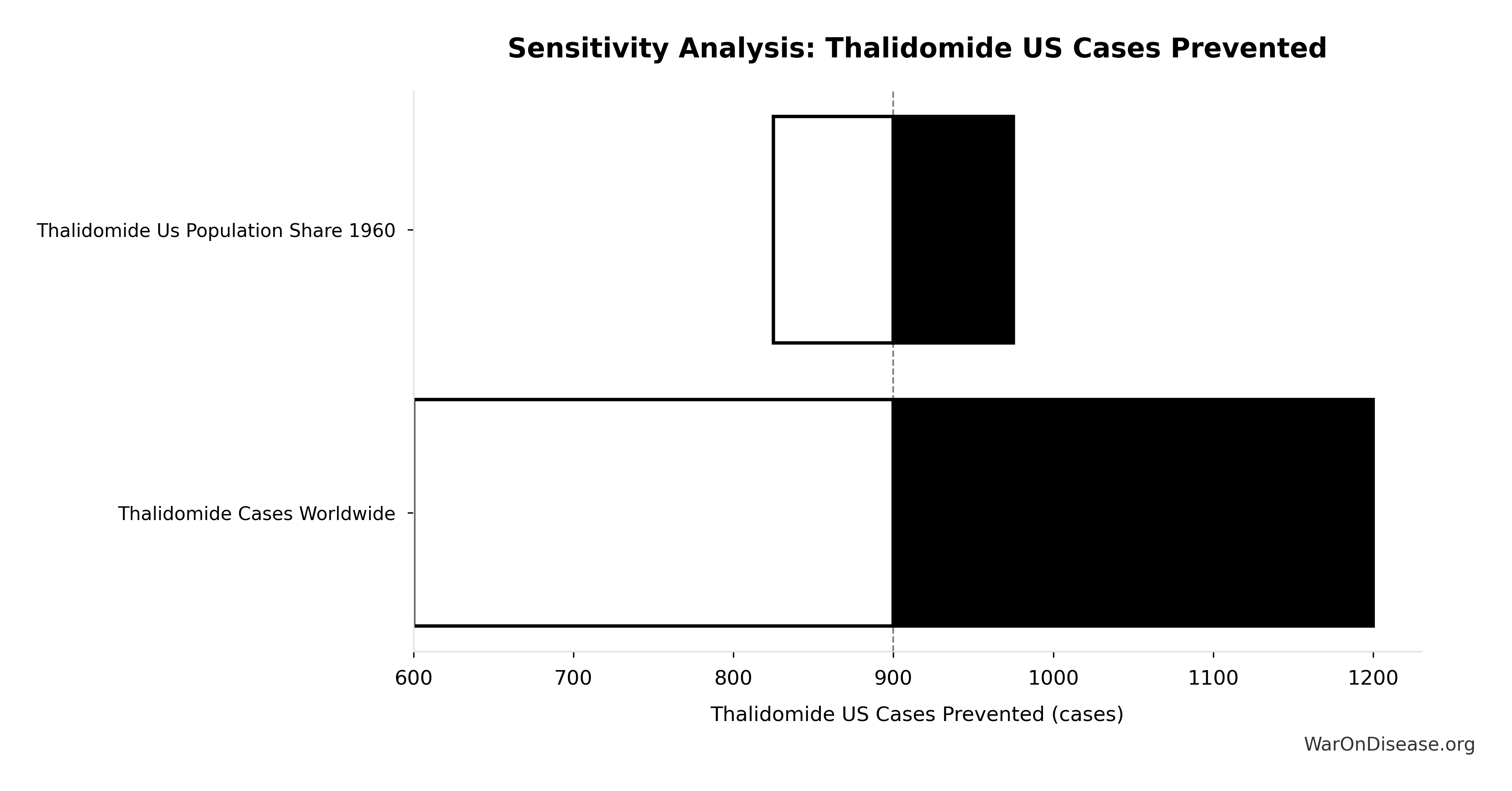
Simulation Results Summary: Thalidomide YLD Per Event
| Statistic | Value |
|---|---|
| Baseline (deterministic) | 13 thousand |
| Mean (expected value) | 13.3 thousand |
| Median (50th percentile) | 12.6 thousand |
| Standard Deviation | 4.5 thousand |
| 90% Range (5th-95th percentile) | [6.94 thousand, 22.6 thousand] |
The histogram shows the distribution of Thalidomide YLD Per Event across 10,000 Monte Carlo simulations. The CDF (right) shows the probability of the outcome exceeding any given value, which is useful for risk assessment.
Exceedance Probability
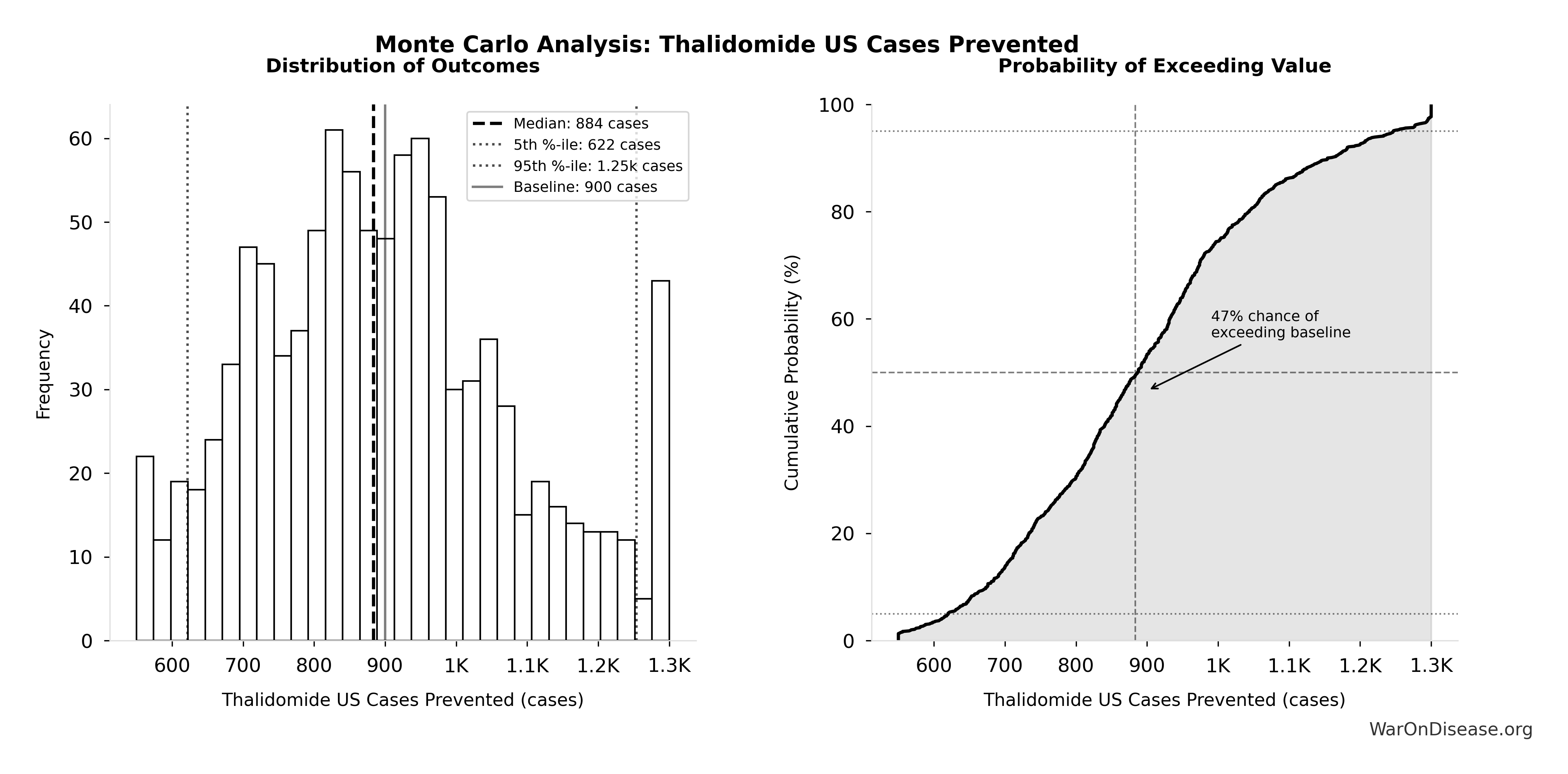
This exceedance probability chart shows the likelihood that Thalidomide YLD Per Event will exceed any given threshold. Higher curves indicate more favorable outcomes with greater certainty.
Thalidomide YLL Per Event: 28.8 thousand years
Note📊 Details
Years of Life Lost per thalidomide event (infant deaths)
Inputs:
- Thalidomide Deaths Per Event 🔢: 360 deaths
\[ \begin{gathered} YLL_{thal} \\ = Deaths_{thal} \times 80 \\ = 360 \times 80 \\ = 28{,}800 \end{gathered} \] where: \[ \begin{gathered} Deaths_{thal} \\ = Rate_{thal,mort} \times N_{thal,US,prevent} \\ = 40\% \times 900 \\ = 360 \end{gathered} \] where: \[ \begin{gathered} N_{thal,US,prevent} \\ = N_{thal,global} \times Pct_{US,1960} \\ = 15{,}000 \times 6\% \\ = 900 \end{gathered} \] ~ Medium confidence
Sensitivity Analysis
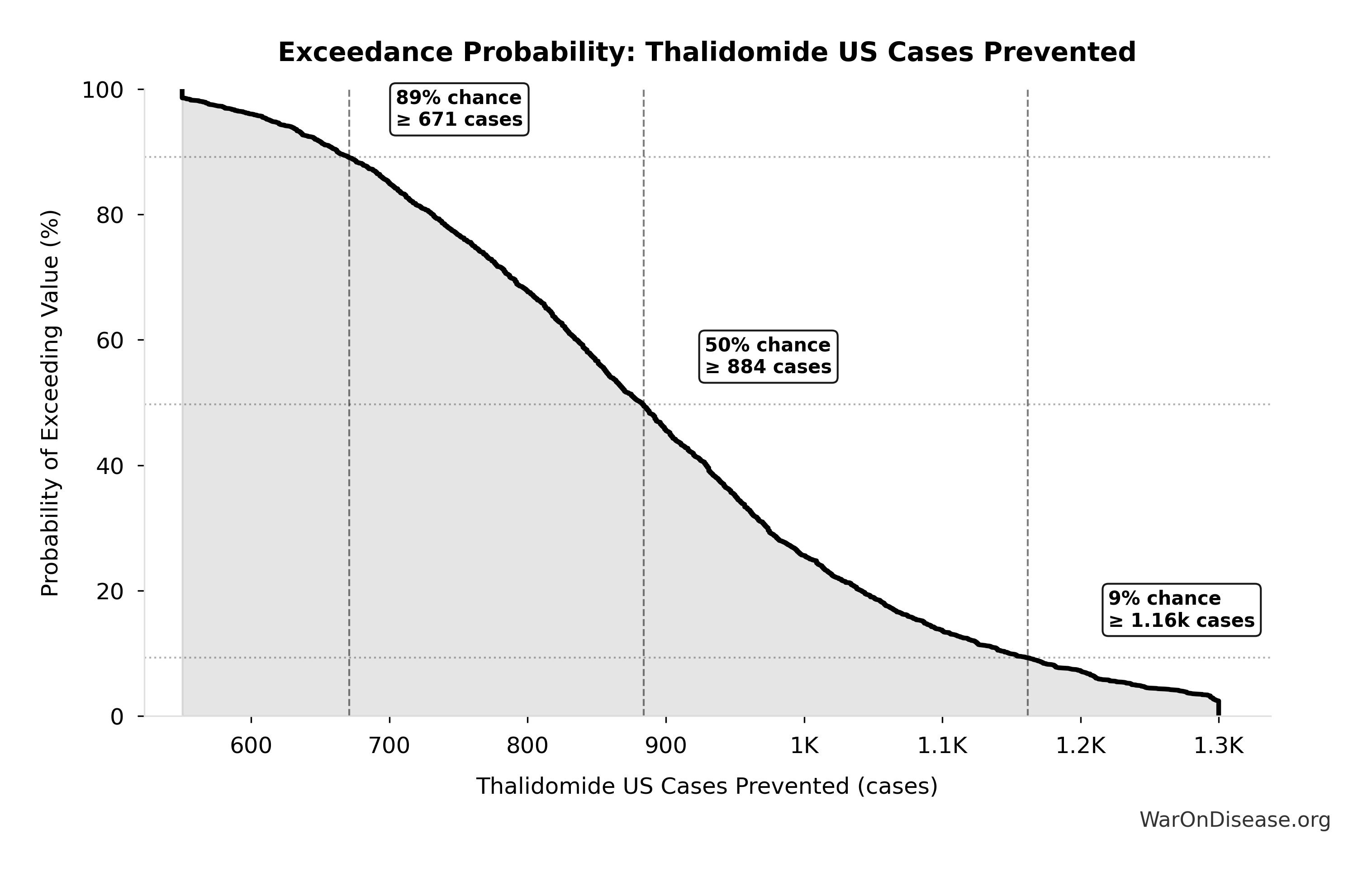
Sensitivity Indices for Thalidomide YLL Per Event
Regression-based sensitivity showing which inputs explain the most variance in the output.
| Input Parameter | Sensitivity Coefficient | Interpretation |
|---|---|---|
| Thalidomide Deaths Per Event (deaths) | 1.0000 | Strong driver |
Interpretation: Standardized coefficients show the change in output (in SD units) per 1 SD change in input. Values near ±1 indicate strong influence; values exceeding ±1 may occur with correlated inputs.
Monte Carlo Distribution
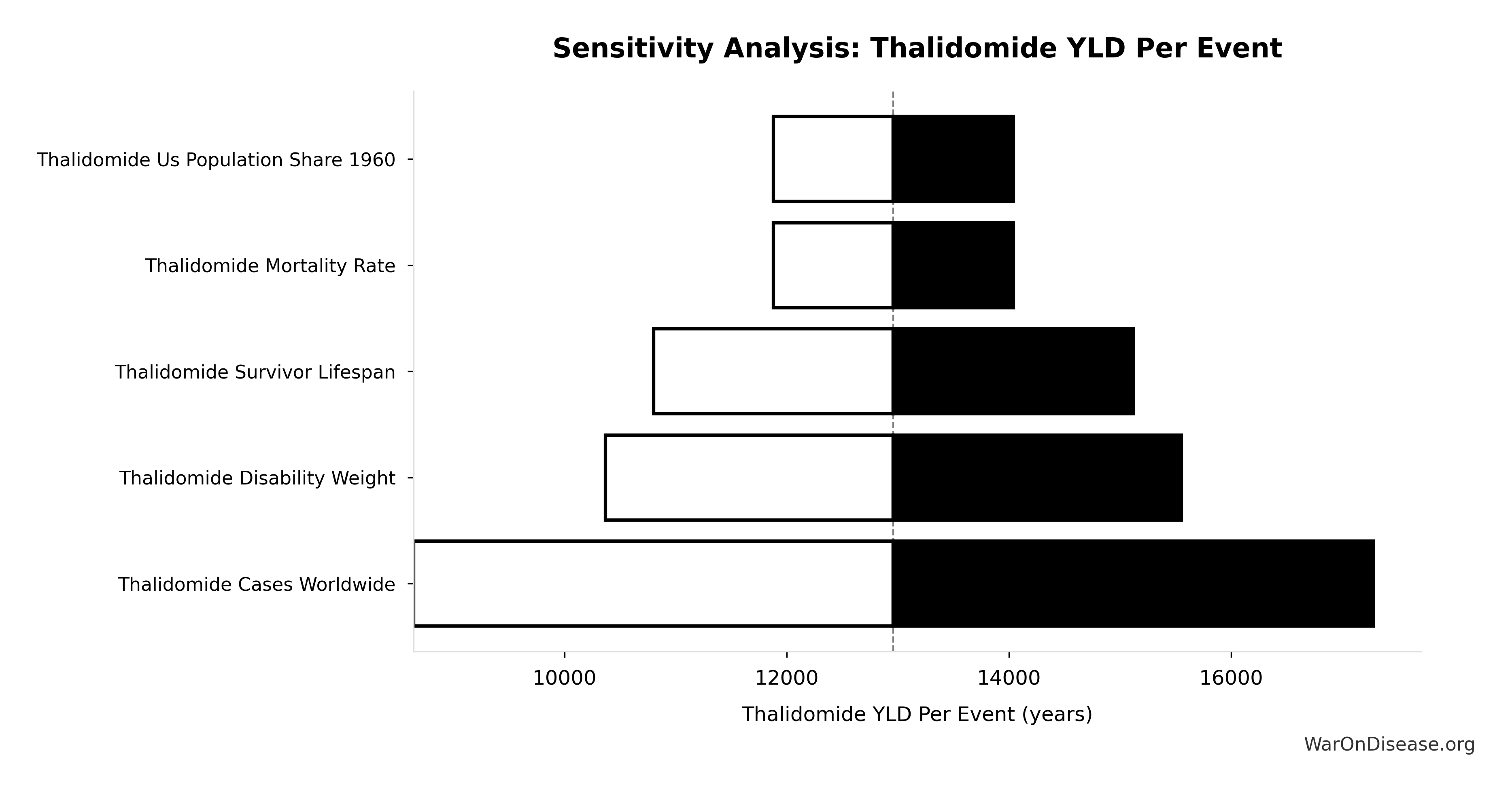
Simulation Results Summary: Thalidomide YLL Per Event
| Statistic | Value |
|---|---|
| Baseline (deterministic) | 28.8 thousand |
| Mean (expected value) | 29.2 thousand |
| Median (50th percentile) | 28.2 thousand |
| Standard Deviation | 7.67 thousand |
| 90% Range (5th-95th percentile) | [17.9 thousand, 44.5 thousand] |
The histogram shows the distribution of Thalidomide YLL Per Event across 10,000 Monte Carlo simulations. The CDF (right) shows the probability of the outcome exceeding any given value, which is useful for risk assessment.
Exceedance Probability
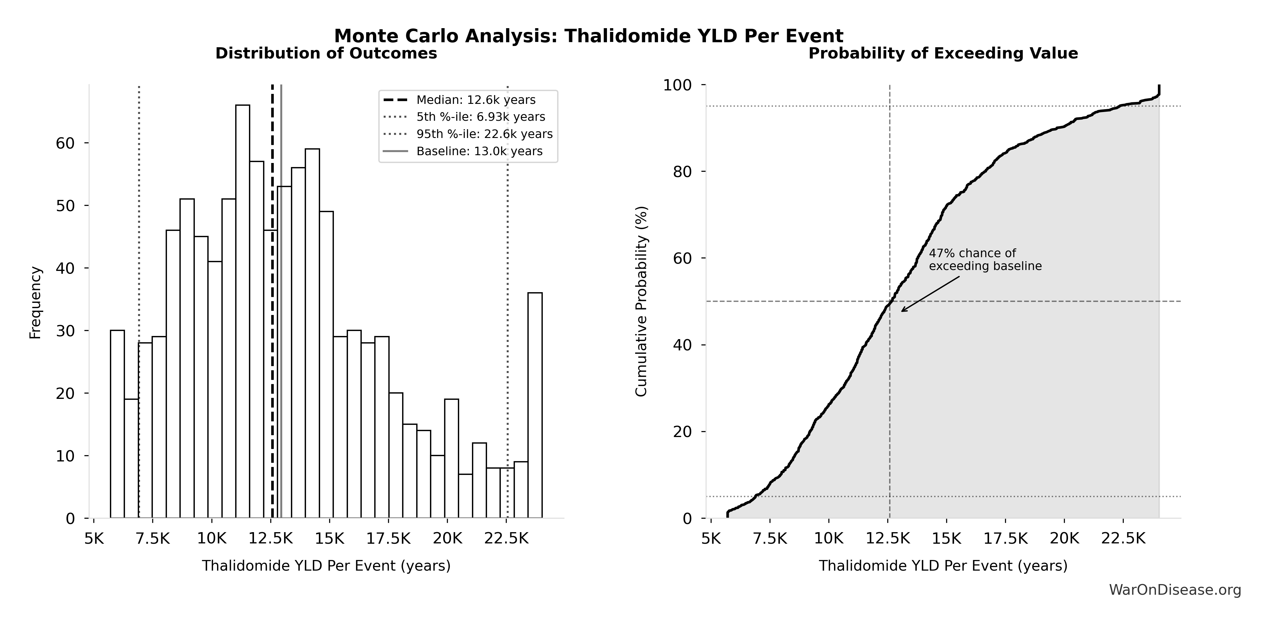
This exceedance probability chart shows the likelihood that Thalidomide YLL Per Event will exceed any given threshold. Higher curves indicate more favorable outcomes with greater certainty.
Annual Funding from 1% of Global Military Spending Redirected to DIH: $27.2B
Note📊 Details
Annual funding from 1% of global military spending redirected to DIH
Inputs:
- Global Military Spending in 2024 📊: $2.72T
- 1% Reduction in Military Spending/War Costs from Treaty: 1%
\[ \begin{gathered} Funding_{treaty} \\ = Spending_{mil} \times Reduce_{treaty} \\ = \$2.72T \times 1\% \\ = \$27.2B \end{gathered} \]
✓ High confidence
Treaty System Benefit Multiplier vs Childhood Vaccination Programs: 11.5x
Note📊 Details
Treaty system benefit multiplier vs childhood vaccination programs
Inputs:
- Estimated Annual Global Economic Benefit from Childhood Vaccination Programs 📊: $15B (SE: ±$4.5B)
- 1% treaty Basic Annual Benefits (Peace + R&D Savings) 🔢: $172B
\[ \begin{gathered} k_{treaty:vax} \\ = \frac{Benefit_{peace+RD}}{Benefit_{vax,ann}} \\ = \frac{\$172B}{\$15B} \\ = 11.5 \end{gathered} \] where: \[ \begin{gathered} Benefit_{peace+RD} \\ = Benefit_{peace,soc} + Benefit_{RD,ann} \\ = \$114B + \$58.6B \\ = \$172B \end{gathered} \] where: \[ \begin{gathered} Benefit_{peace,soc} \\ = Cost_{war,total} \times Reduce_{treaty} \\ = \$11.4T \times 1\% \\ = \$114B \end{gathered} \] where: \[ \begin{gathered} Cost_{war,total} \\ = Cost_{war,direct} + Cost_{war,indirect} \\ = \$7.66T + \$3.7T \\ = \$11.4T \end{gathered} \] where: \[ \begin{gathered} Cost_{war,direct} \\ = Loss_{life,conflict} + Damage_{infra,total} \\ + Disruption_{trade} + Spending_{mil} \\ = \$2.45T + \$1.88T + \$616B + \$2.72T \\ = \$7.66T \end{gathered} \] where: \[ \begin{gathered} Loss_{life,conflict} \\ = Cost_{combat,human} + Cost_{state,human} \\ + Cost_{terror,human} \\ = \$2.34T + \$27B + \$83B \\ = \$2.45T \end{gathered} \] where: \[ \begin{gathered} Cost_{combat,human} \\ = Deaths_{combat} \times VSL \\ = 234{,}000 \times \$10M \\ = \$2.34T \end{gathered} \] where: \[ \begin{gathered} Cost_{state,human} \\ = Deaths_{state} \times VSL \\ = 2{,}700 \times \$10M \\ = \$27B \end{gathered} \] where: \[ \begin{gathered} Cost_{terror,human} \\ = Deaths_{terror} \times VSL \\ = 8{,}300 \times \$10M \\ = \$83B \end{gathered} \] where: \[ \begin{gathered} Damage_{infra,total} \\ = Damage_{comms} + Damage_{edu} + Damage_{energy} \\ + Damage_{health} + Damage_{transport} + Damage_{water} \\ = \$298B + \$234B + \$422B + \$166B + \$487B + \$268B \\ = \$1.88T \end{gathered} \] where: \[ \begin{gathered} Disruption_{trade} \\ = Disruption_{currency} + Disruption_{energy} \\ + Disruption_{shipping} + Disruption_{supply} \\ = \$57.4B + \$125B + \$247B + \$187B \\ = \$616B \end{gathered} \] where: \[ \begin{gathered} Cost_{war,indirect} \\ = Damage_{env} + Loss_{growth,mil} + Loss_{capital,conflict} \\ + Cost_{psych} + Cost_{refugee} + Cost_{vet} \\ = \$100B + \$2.72T + \$300B + \$232B + \$150B + \$200B \\ = \$3.7T \end{gathered} \] where: \[ \begin{gathered} Benefit_{RD,ann} \\ = Spending_{trials} \times Reduce_{pct} \\ = \$60B \times 97.7\% \\ = \$58.6B \end{gathered} \] where: \[ \begin{gathered} Reduce_{pct} \\ = 1 - \frac{Cost_{pragmatic,pt}}{Cost_{P3,pt}} \\ = 1 - \frac{\$929}{\$41K} \\ = 97.7\% \end{gathered} \] ✓ High confidence
Sensitivity Analysis

Sensitivity Indices for Treaty System Benefit Multiplier vs Childhood Vaccination Programs
Regression-based sensitivity showing which inputs explain the most variance in the output.
| Input Parameter | Sensitivity Coefficient | Interpretation |
|---|---|---|
| Estimated Annual Global Economic Benefit from Childhood Vaccination Programs (USD/year) | -1.1963 | Strong driver |
| 1% treaty Basic Annual Benefits (Peace + R&D Savings) (USD/year) | 0.3259 | Moderate driver |
Interpretation: Standardized coefficients show the change in output (in SD units) per 1 SD change in input. Values near ±1 indicate strong influence; values exceeding ±1 may occur with correlated inputs.
Monte Carlo Distribution
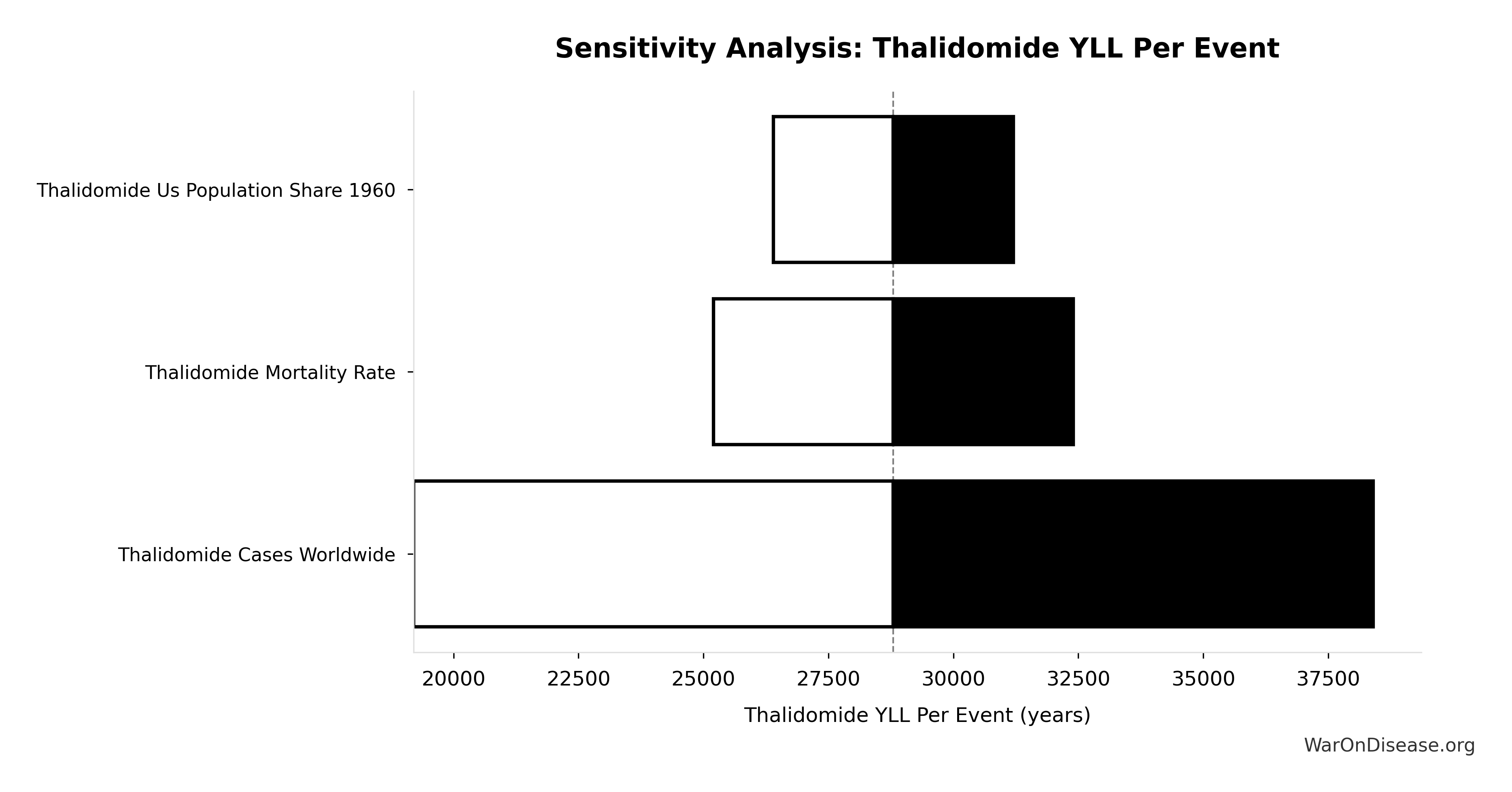
Simulation Results Summary: Treaty System Benefit Multiplier vs Childhood Vaccination Programs
| Statistic | Value |
|---|---|
| Baseline (deterministic) | 11.5x |
| Mean (expected value) | 12.1x |
| Median (50th percentile) | 11.8x |
| Standard Deviation | 2.28x |
| 90% Range (5th-95th percentile) | [9x, 16.1x] |
The histogram shows the distribution of Treaty System Benefit Multiplier vs Childhood Vaccination Programs across 10,000 Monte Carlo simulations. The CDF (right) shows the probability of the outcome exceeding any given value, which is useful for risk assessment.
Exceedance Probability

This exceedance probability chart shows the likelihood that Treaty System Benefit Multiplier vs Childhood Vaccination Programs will exceed any given threshold. Higher curves indicate more favorable outcomes with greater certainty.
Total 1% Treaty Campaign Cost: $1B
Note📊 Details
Total treaty campaign cost (100% VICTORY Incentive Alignment Bonds)
Inputs:
- Viral Referendum Budget: $250M (95% CI: $150M - $410M)
- Political Lobbying Campaign: Direct Lobbying, Super Pacs, Opposition Research, Staff, Legal/Compliance: $650M (95% CI: $325M - $1.3B)
- Reserve Fund / Contingency Buffer: $100M (95% CI: $20M - $150M)
\[ \begin{gathered} Cost_{campaign} \\ = Budget_{viral,base} + Budget_{lobby,treaty} \\ + Budget_{reserve} \\ = \$250M + \$650M + \$100M \\ = \$1B \end{gathered} \]
✓ High confidence
Sensitivity Analysis
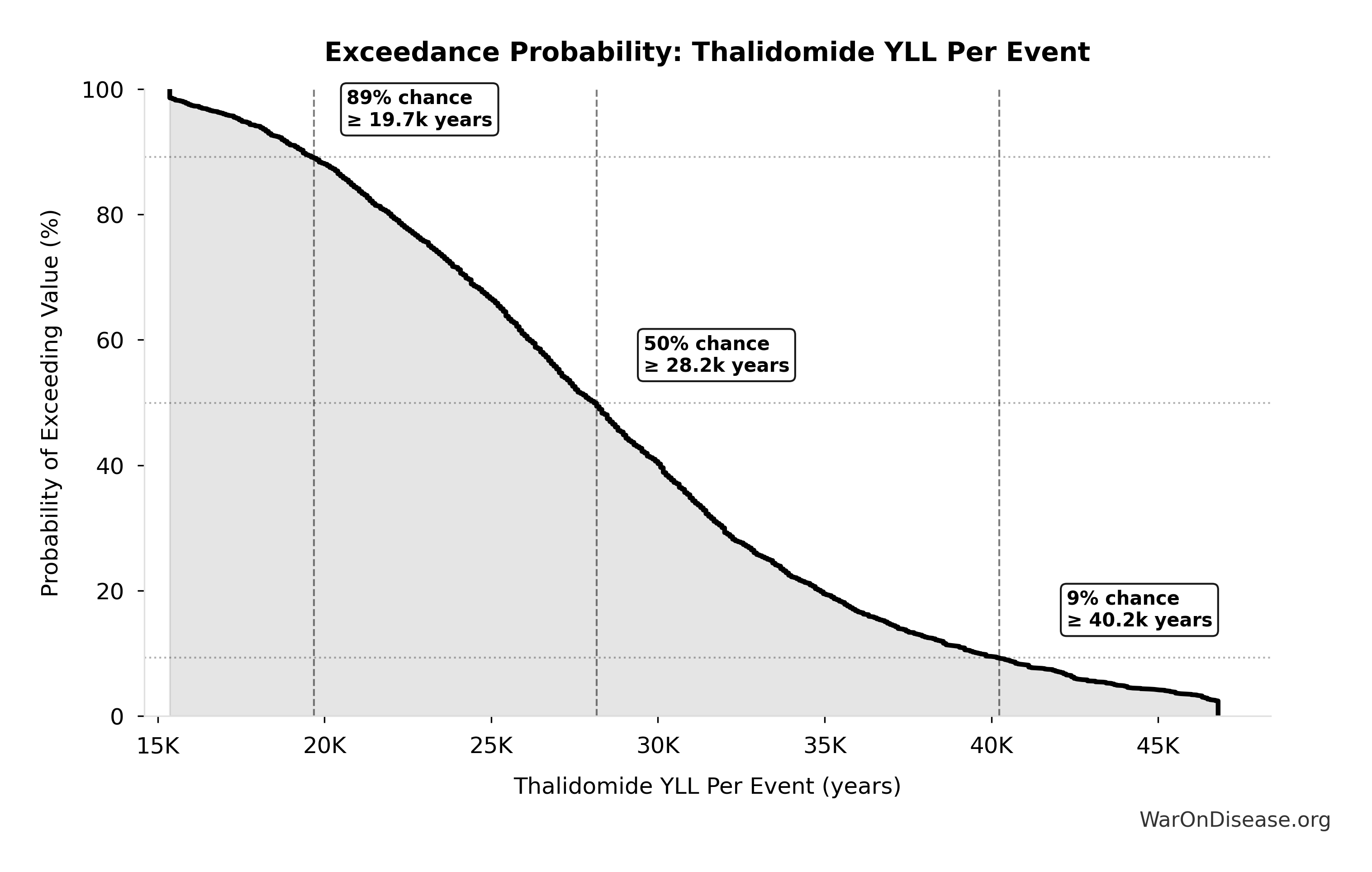
Sensitivity Indices for Total 1% Treaty Campaign Cost
Regression-based sensitivity showing which inputs explain the most variance in the output.
| Input Parameter | Sensitivity Coefficient | Interpretation |
|---|---|---|
| Political Lobbying Campaign: Direct Lobbying, Super Pacs, Opposition Research, Staff, Legal/Compliance (USD) | 0.9016 | Strong driver |
| Reserve Fund / Contingency Buffer (USD) | 0.1026 | Weak driver |
Interpretation: Standardized coefficients show the change in output (in SD units) per 1 SD change in input. Values near ±1 indicate strong influence; values exceeding ±1 may occur with correlated inputs.
Monte Carlo Distribution
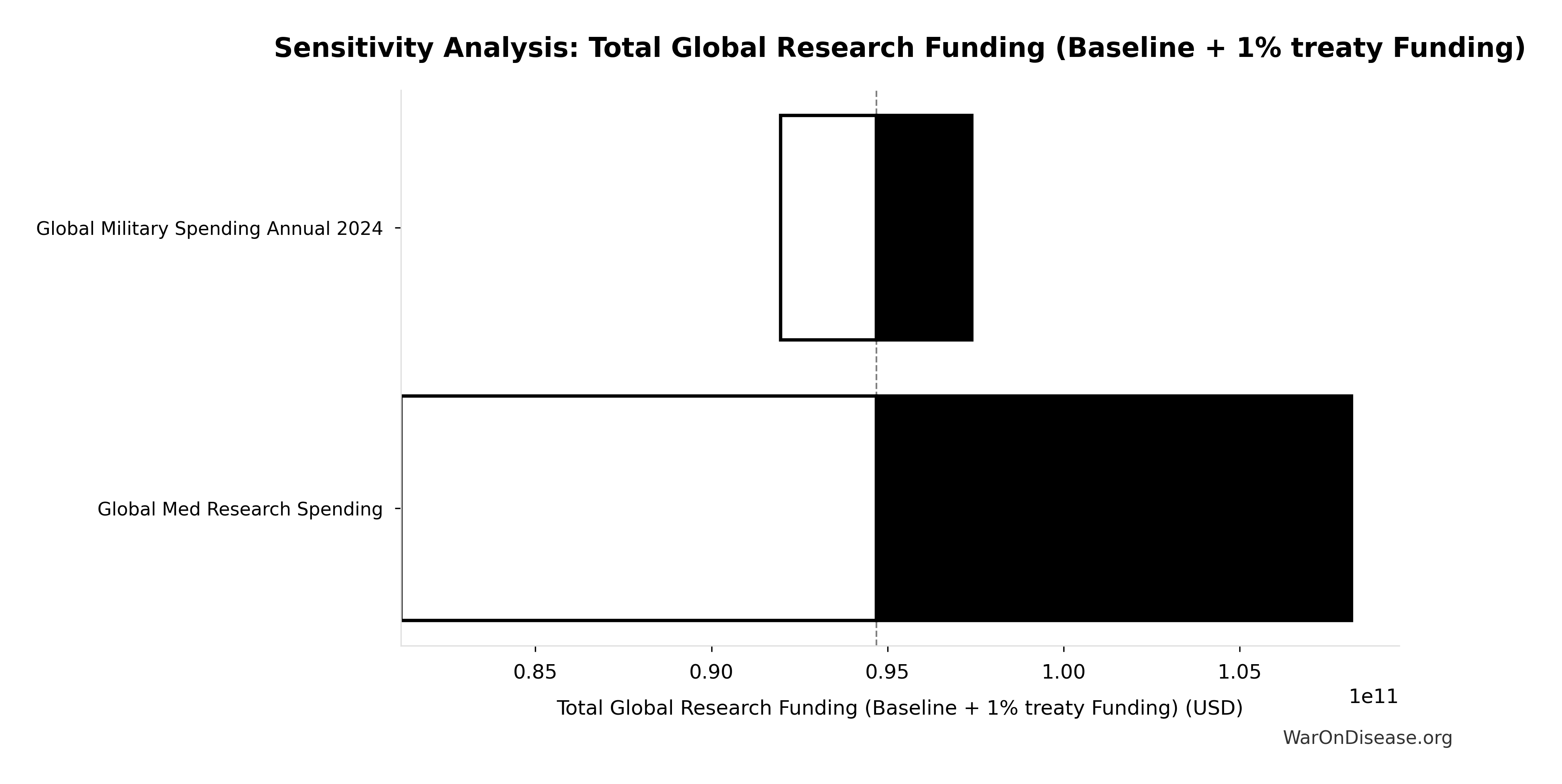
Simulation Results Summary: Total 1% Treaty Campaign Cost
| Statistic | Value |
|---|---|
| Baseline (deterministic) | $1B |
| Mean (expected value) | $996M |
| Median (50th percentile) | $949M |
| Standard Deviation | $276M |
| 90% Range (5th-95th percentile) | [$632M, $1.51B] |
The histogram shows the distribution of Total 1% Treaty Campaign Cost across 10,000 Monte Carlo simulations. The CDF (right) shows the probability of the outcome exceeding any given value, which is useful for risk assessment.
Exceedance Probability
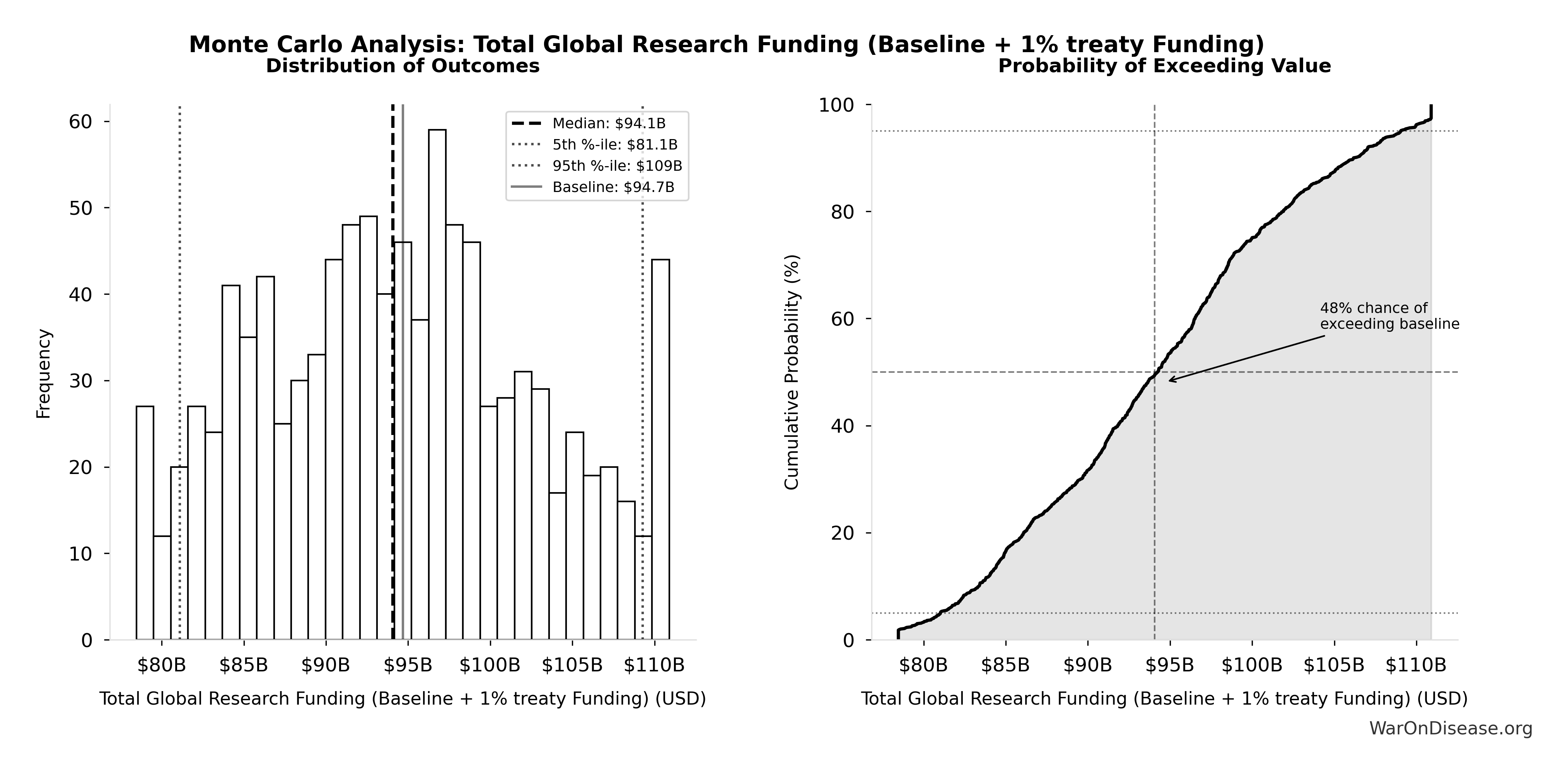
This exceedance probability chart shows the likelihood that Total 1% Treaty Campaign Cost will exceed any given threshold. Higher curves indicate more favorable outcomes with greater certainty.
Target Voting Bloc Size for Campaign: 280 million of people
Note📊 Details
Target voting bloc size for campaign (3.5% of global population - critical mass for social change). Wide CI reflects uncertainty in applying Chenoweth’s national threshold to global treaty adoption.
Inputs:
- Global Population in 2024 📊: 8 billion of people (95% CI: 7.8 billion of people - 8.2 billion of people)
- Critical Mass Threshold for Social Change 📊: 3.5% (95% CI: 1% - 10%)
\[ \begin{gathered} N_{voters,target} \\ = Pop_{global} \times Threshold_{activism} \\ = 8B \times 3.5\% \\ = 280M \end{gathered} \]
✓ High confidence
Sensitivity Analysis
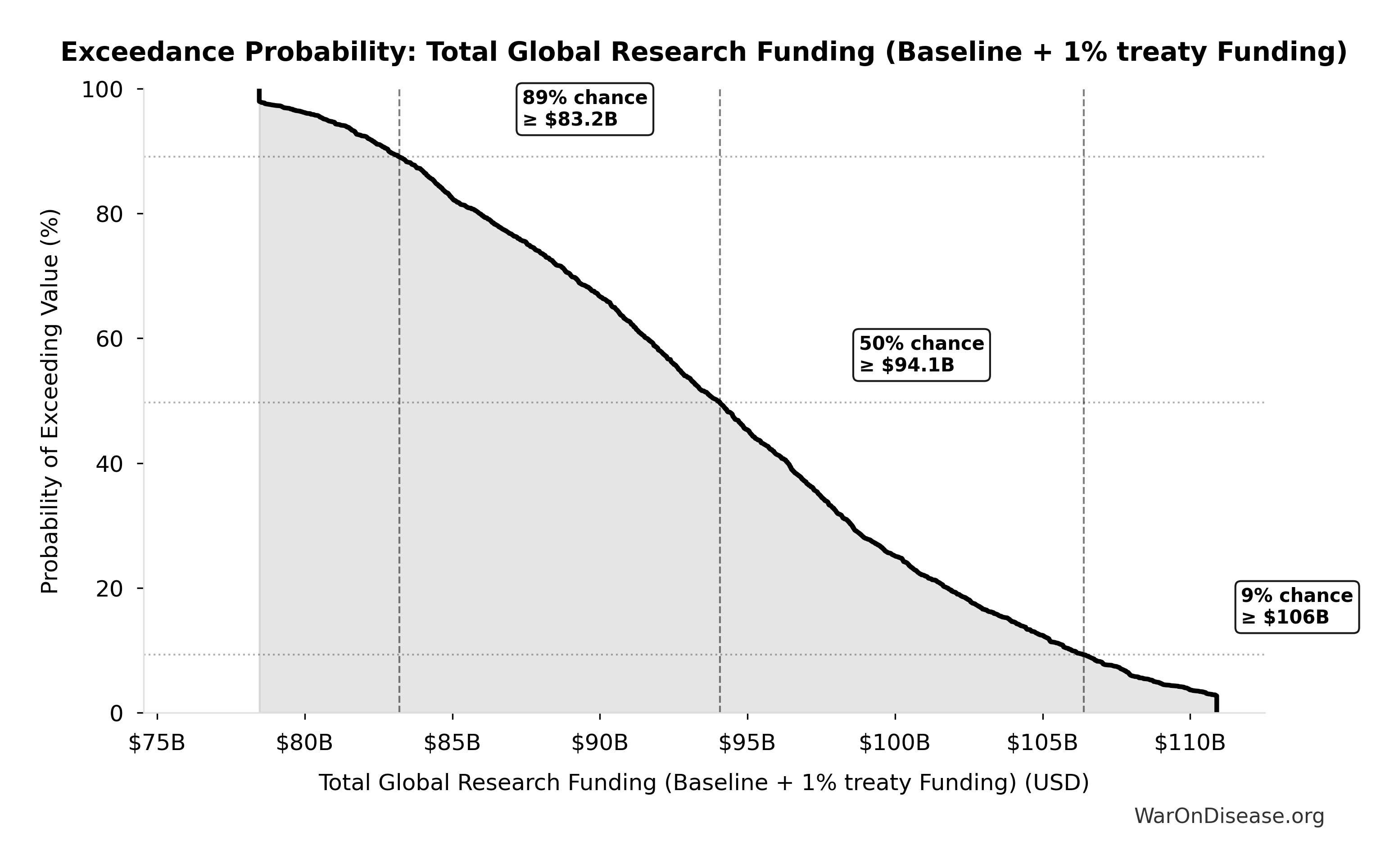
Sensitivity Indices for Target Voting Bloc Size for Campaign
Regression-based sensitivity showing which inputs explain the most variance in the output.
| Input Parameter | Sensitivity Coefficient | Interpretation |
|---|---|---|
| Critical Mass Threshold for Social Change (percent) | 1.0166 | Strong driver |
| Global Population in 2024 (of people) | -0.0177 | Minimal effect |
Interpretation: Standardized coefficients show the change in output (in SD units) per 1 SD change in input. Values near ±1 indicate strong influence; values exceeding ±1 may occur with correlated inputs.
Monte Carlo Distribution
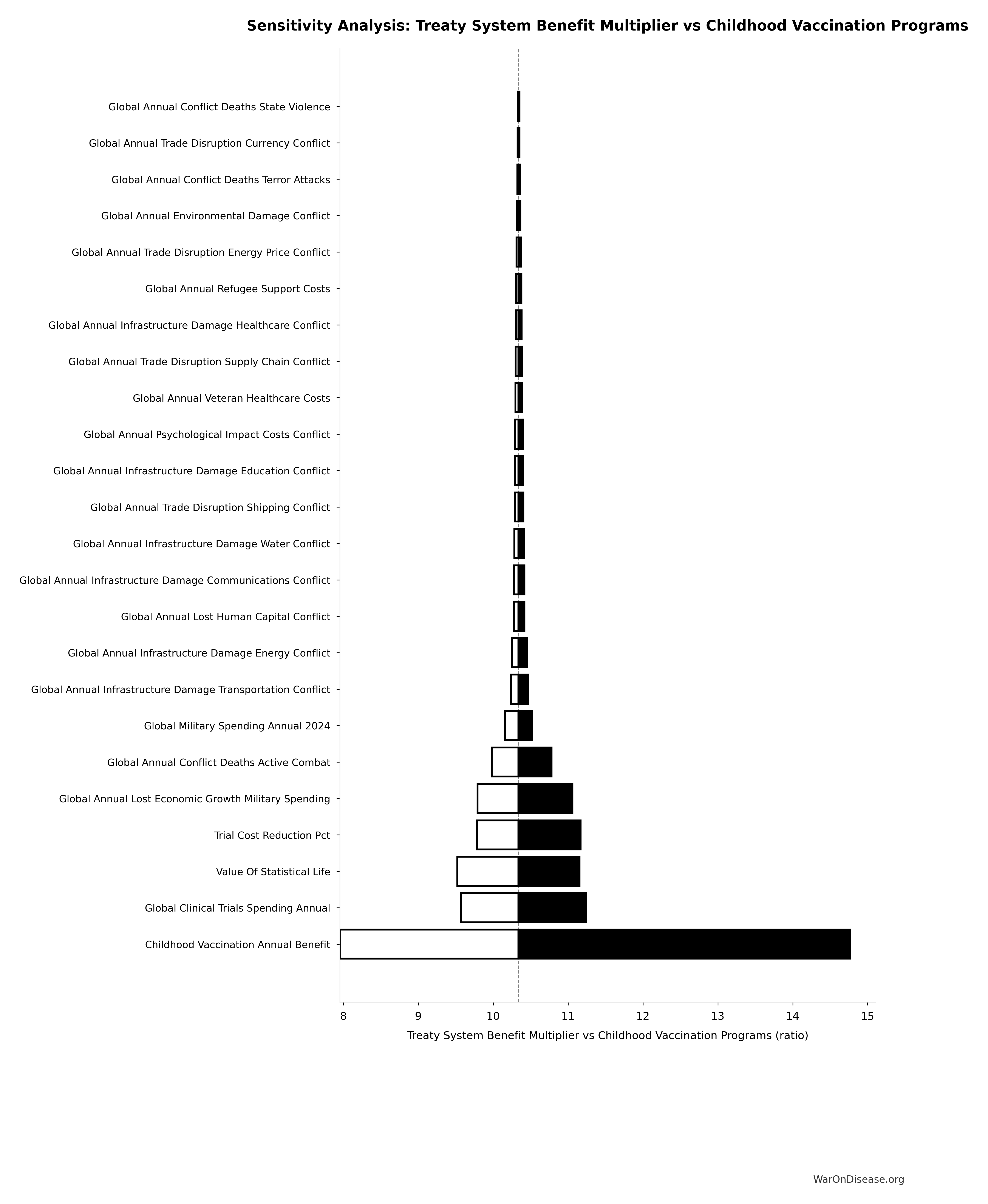
Simulation Results Summary: Target Voting Bloc Size for Campaign
| Statistic | Value |
|---|---|
| Baseline (deterministic) | 280 million |
| Mean (expected value) | 277 million |
| Median (50th percentile) | 232 million |
| Standard Deviation | 169 million |
| 90% Range (5th-95th percentile) | [84.2 million, 639 million] |
The histogram shows the distribution of Target Voting Bloc Size for Campaign across 10,000 Monte Carlo simulations. The CDF (right) shows the probability of the outcome exceeding any given value, which is useful for risk assessment.
Exceedance Probability
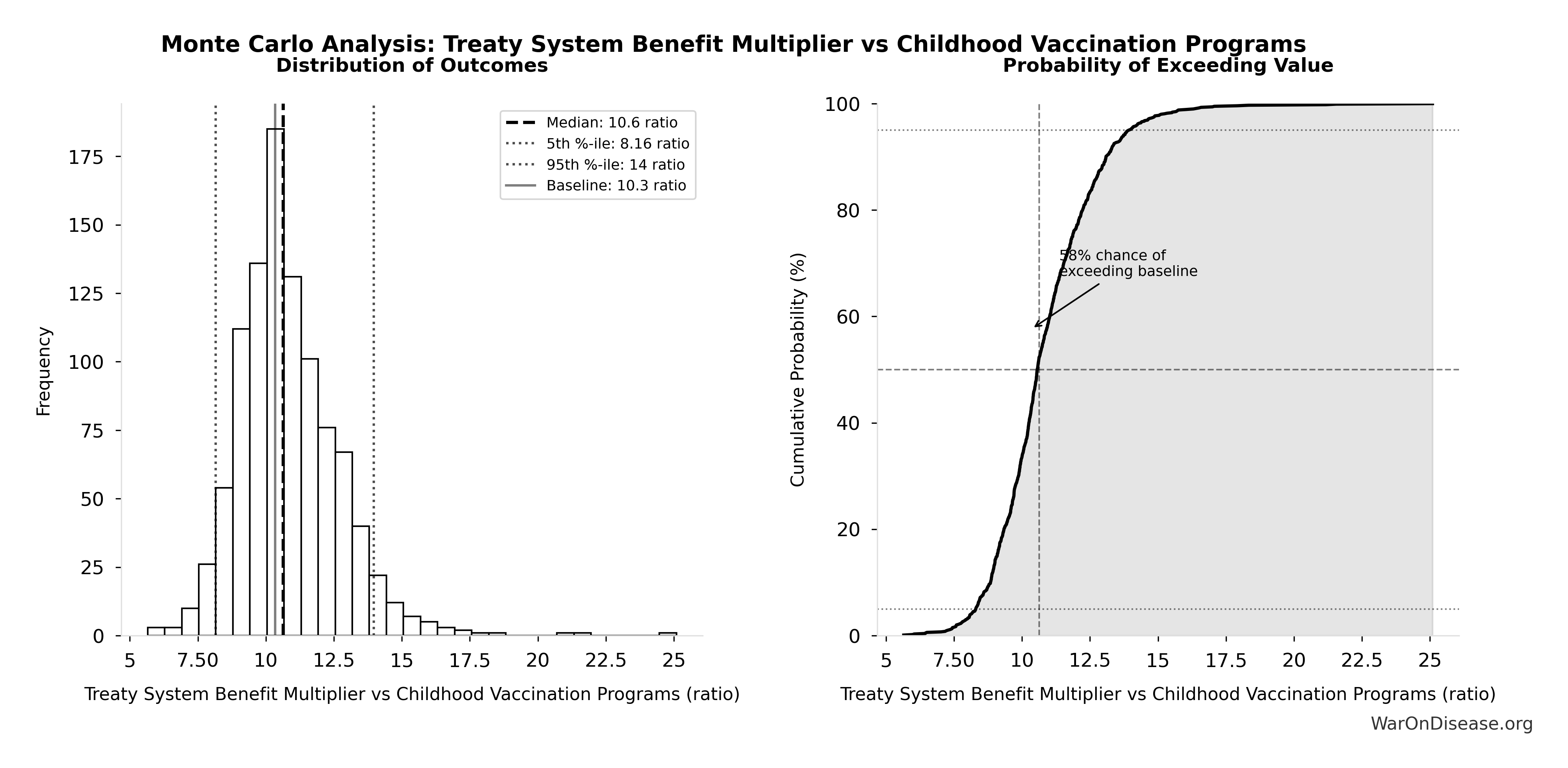
This exceedance probability chart shows the likelihood that Target Voting Bloc Size for Campaign will exceed any given threshold. Higher curves indicate more favorable outcomes with greater certainty.
Cost per DALY Averted (Elimination of Efficacy Lag Plus Earlier Treatment Discovery from Increased Trial Throughput): $0.00177
Note📊 Details
Cost per DALY averted from elimination of efficacy lag plus earlier treatment discovery from increased trial throughput. Only counts campaign cost; ignores economic benefits from funding and R&D savings.
Inputs:
- Total 1% Treaty Campaign Cost 🔢: $1B
- Total DALYs from Elimination of Efficacy Lag Plus Earlier Treatment Discovery from Higher Trial Throughput 🔢: 565 billion DALYs
\[ \begin{gathered} Cost_{treaty,DALY} \\ = \frac{Cost_{campaign}}{DALYs_{max}} \\ = \frac{\$1B}{565B} \\ = \$0.00177 \end{gathered} \] where: \[ \begin{gathered} Cost_{campaign} \\ = Budget_{viral,base} + Budget_{lobby,treaty} \\ + Budget_{reserve} \\ = \$250M + \$650M + \$100M \\ = \$1B \end{gathered} \] where: \[ \begin{gathered} DALYs_{max} \\ = DALYs_{global,ann} \times Pct_{avoid,DALY} \times T_{accel,max} \\ = 2.88B \times 92.6\% \times 212 \\ = 565B \end{gathered} \] where: \[ T_{accel,max} = T_{accel} + T_{lag} = 204 + 8.2 = 212 \] where: \[ \begin{gathered} T_{accel} \\ = T_{first,SQ} \times \left(1 - \frac{1}{k_{capacity}}\right) \\ = 222 \times \left(1 - \frac{1}{12.3}\right) \\ = 204 \end{gathered} \] where: \[ \begin{gathered} T_{first,SQ} \\ = T_{queue,SQ} \times 0.5 \\ = 443 \times 0.5 \\ = 222 \end{gathered} \] where: \[ \begin{gathered} T_{queue,SQ} \\ = \frac{N_{untreated}}{Treatments_{new,ann}} \\ = \frac{6{,}650}{15} \\ = 443 \end{gathered} \] where: \[ \begin{gathered} N_{untreated} \\ = N_{rare} \times 0.95 \\ = 7{,}000 \times 0.95 \\ = 6{,}650 \end{gathered} \] where: \[ \begin{gathered} k_{capacity} \\ = \frac{N_{fundable,dFDA}}{Slots_{curr}} \\ = \frac{23.4M}{1.9M} \\ = 12.3 \end{gathered} \] where: \[ \begin{gathered} N_{fundable,dFDA} \\ = \frac{Subsidies_{dFDA,ann}}{Cost_{pragmatic,pt}} \\ = \frac{\$21.8B}{\$929} \\ = 23.4M \end{gathered} \] where: \[ \begin{gathered} Subsidies_{dFDA,ann} \\ = Funding_{dFDA,ann} - OPEX_{dFDA} \\ = \$21.8B - \$40M \\ = \$21.8B \end{gathered} \] where: \[ \begin{gathered} OPEX_{dFDA} \\ = Cost_{platform} + Cost_{staff} + Cost_{infra} \\ + Cost_{regulatory} + Cost_{community} \\ = \$15M + \$10M + \$8M + \$5M + \$2M \\ = \$40M \end{gathered} \] ✓ High confidence
Sensitivity Analysis
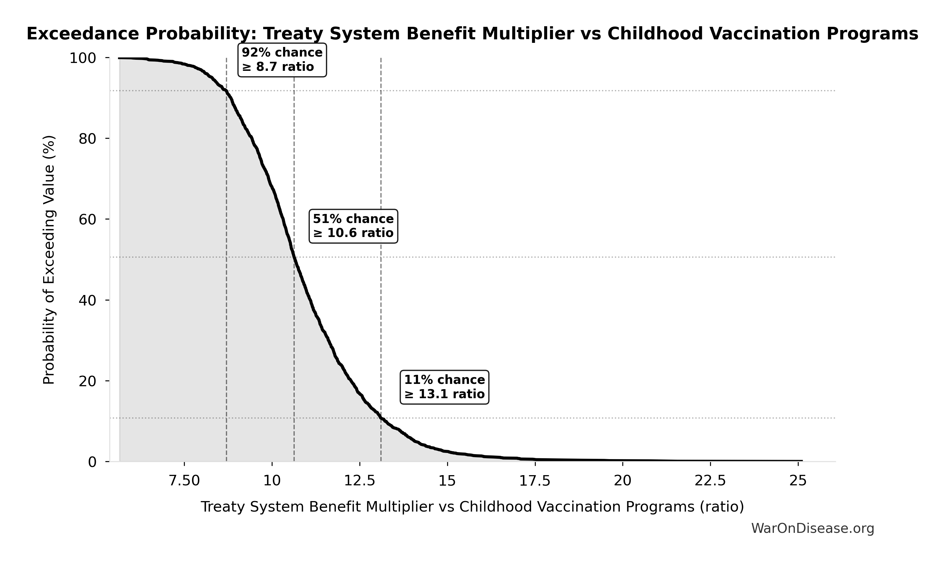
Sensitivity Indices for Cost per DALY Averted (Elimination of Efficacy Lag Plus Earlier Treatment Discovery from Increased Trial Throughput)
Regression-based sensitivity showing which inputs explain the most variance in the output.
| Input Parameter | Sensitivity Coefficient | Interpretation |
|---|---|---|
| Total 1% Treaty Campaign Cost (USD) | 0.6487 | Strong driver |
| Total DALYs from Elimination of Efficacy Lag Plus Earlier Treatment Discovery from Higher Trial Throughput (DALYs) | -0.3322 | Moderate driver |
Interpretation: Standardized coefficients show the change in output (in SD units) per 1 SD change in input. Values near ±1 indicate strong influence; values exceeding ±1 may occur with correlated inputs.
Monte Carlo Distribution
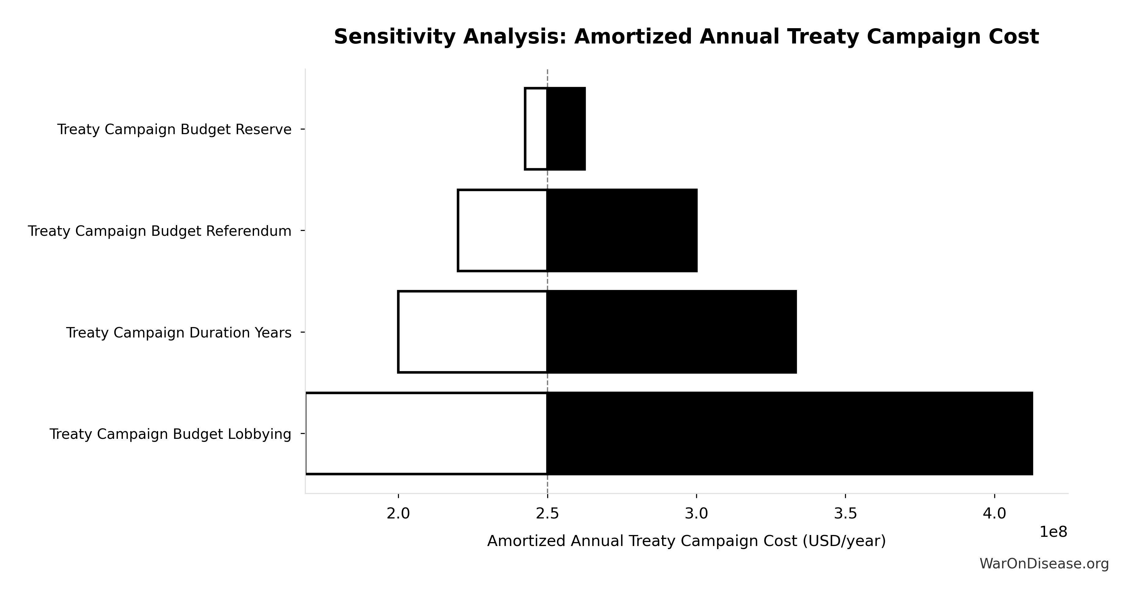
Simulation Results Summary: Cost per DALY Averted (Elimination of Efficacy Lag Plus Earlier Treatment Discovery from Increased Trial Throughput)
| Statistic | Value |
|---|---|
| Baseline (deterministic) | $0.00177 |
| Mean (expected value) | $0.00186 |
| Median (50th percentile) | $0.00156 |
| Standard Deviation | $0.00109 |
| 90% Range (5th-95th percentile) | [$0.000715, $0.00412] |
The histogram shows the distribution of Cost per DALY Averted (Elimination of Efficacy Lag Plus Earlier Treatment Discovery from Increased Trial Throughput) across 10,000 Monte Carlo simulations. The CDF (right) shows the probability of the outcome exceeding any given value, which is useful for risk assessment.
Exceedance Probability
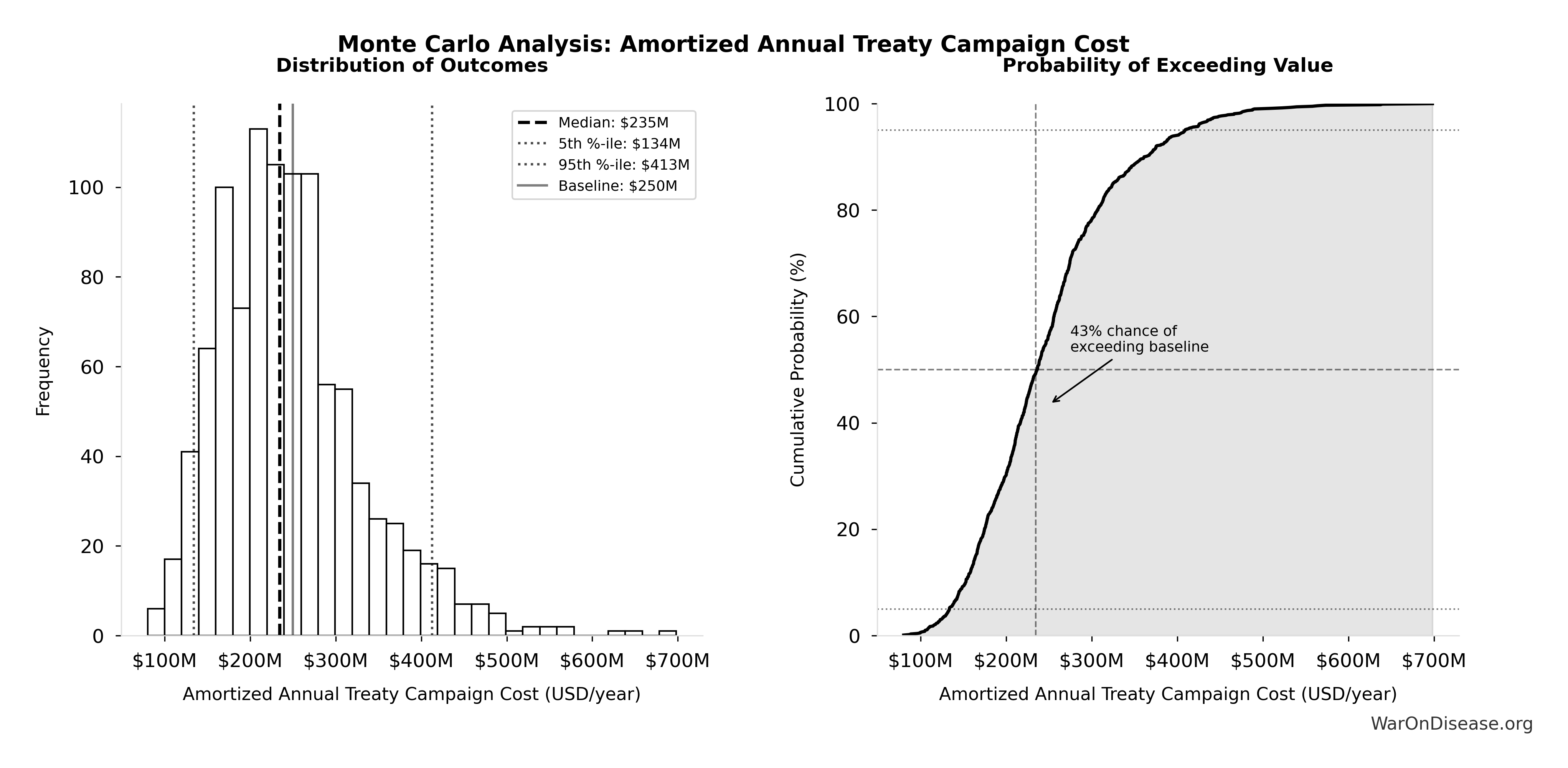
This exceedance probability chart shows the likelihood that Cost per DALY Averted (Elimination of Efficacy Lag Plus Earlier Treatment Discovery from Increased Trial Throughput) will exceed any given threshold. Higher curves indicate more favorable outcomes with greater certainty.
Expected Cost per DALY (Risk-Adjusted): $0.177
Note📊 Details
Expected cost per DALY accounting for political success probability uncertainty. Monte Carlo samples from beta(0.1%, 10%) distribution. At the conservative 1% estimate, this is still more cost-effective than bed nets ($89.0/DALY).
Inputs:
- Cost per DALY Averted (Elimination of Efficacy Lag Plus Earlier Treatment Discovery from Increased Trial Throughput) 🔢: $0.00177
- Political Success Probability 📊: 1% (95% CI: 0.1% - 10%)
\[ \begin{gathered} E[Cost_{DALY}] \\ = \frac{Cost_{treaty,DALY}}{P_{success}} \\ = \frac{\$0.00177}{1\%} \\ = \$0.177 \end{gathered} \] where: \[ \begin{gathered} Cost_{treaty,DALY} \\ = \frac{Cost_{campaign}}{DALYs_{max}} \\ = \frac{\$1B}{565B} \\ = \$0.00177 \end{gathered} \] where: \[ \begin{gathered} Cost_{campaign} \\ = Budget_{viral,base} + Budget_{lobby,treaty} \\ + Budget_{reserve} \\ = \$250M + \$650M + \$100M \\ = \$1B \end{gathered} \] where: \[ \begin{gathered} DALYs_{max} \\ = DALYs_{global,ann} \times Pct_{avoid,DALY} \times T_{accel,max} \\ = 2.88B \times 92.6\% \times 212 \\ = 565B \end{gathered} \] where: \[ T_{accel,max} = T_{accel} + T_{lag} = 204 + 8.2 = 212 \] where: \[ \begin{gathered} T_{accel} \\ = T_{first,SQ} \times \left(1 - \frac{1}{k_{capacity}}\right) \\ = 222 \times \left(1 - \frac{1}{12.3}\right) \\ = 204 \end{gathered} \] where: \[ \begin{gathered} T_{first,SQ} \\ = T_{queue,SQ} \times 0.5 \\ = 443 \times 0.5 \\ = 222 \end{gathered} \] where: \[ \begin{gathered} T_{queue,SQ} \\ = \frac{N_{untreated}}{Treatments_{new,ann}} \\ = \frac{6{,}650}{15} \\ = 443 \end{gathered} \] where: \[ \begin{gathered} N_{untreated} \\ = N_{rare} \times 0.95 \\ = 7{,}000 \times 0.95 \\ = 6{,}650 \end{gathered} \] where: \[ \begin{gathered} k_{capacity} \\ = \frac{N_{fundable,dFDA}}{Slots_{curr}} \\ = \frac{23.4M}{1.9M} \\ = 12.3 \end{gathered} \] where: \[ \begin{gathered} N_{fundable,dFDA} \\ = \frac{Subsidies_{dFDA,ann}}{Cost_{pragmatic,pt}} \\ = \frac{\$21.8B}{\$929} \\ = 23.4M \end{gathered} \] where: \[ \begin{gathered} Subsidies_{dFDA,ann} \\ = Funding_{dFDA,ann} - OPEX_{dFDA} \\ = \$21.8B - \$40M \\ = \$21.8B \end{gathered} \] where: \[ \begin{gathered} OPEX_{dFDA} \\ = Cost_{platform} + Cost_{staff} + Cost_{infra} \\ + Cost_{regulatory} + Cost_{community} \\ = \$15M + \$10M + \$8M + \$5M + \$2M \\ = \$40M \end{gathered} \] ? Low confidence
Sensitivity Analysis
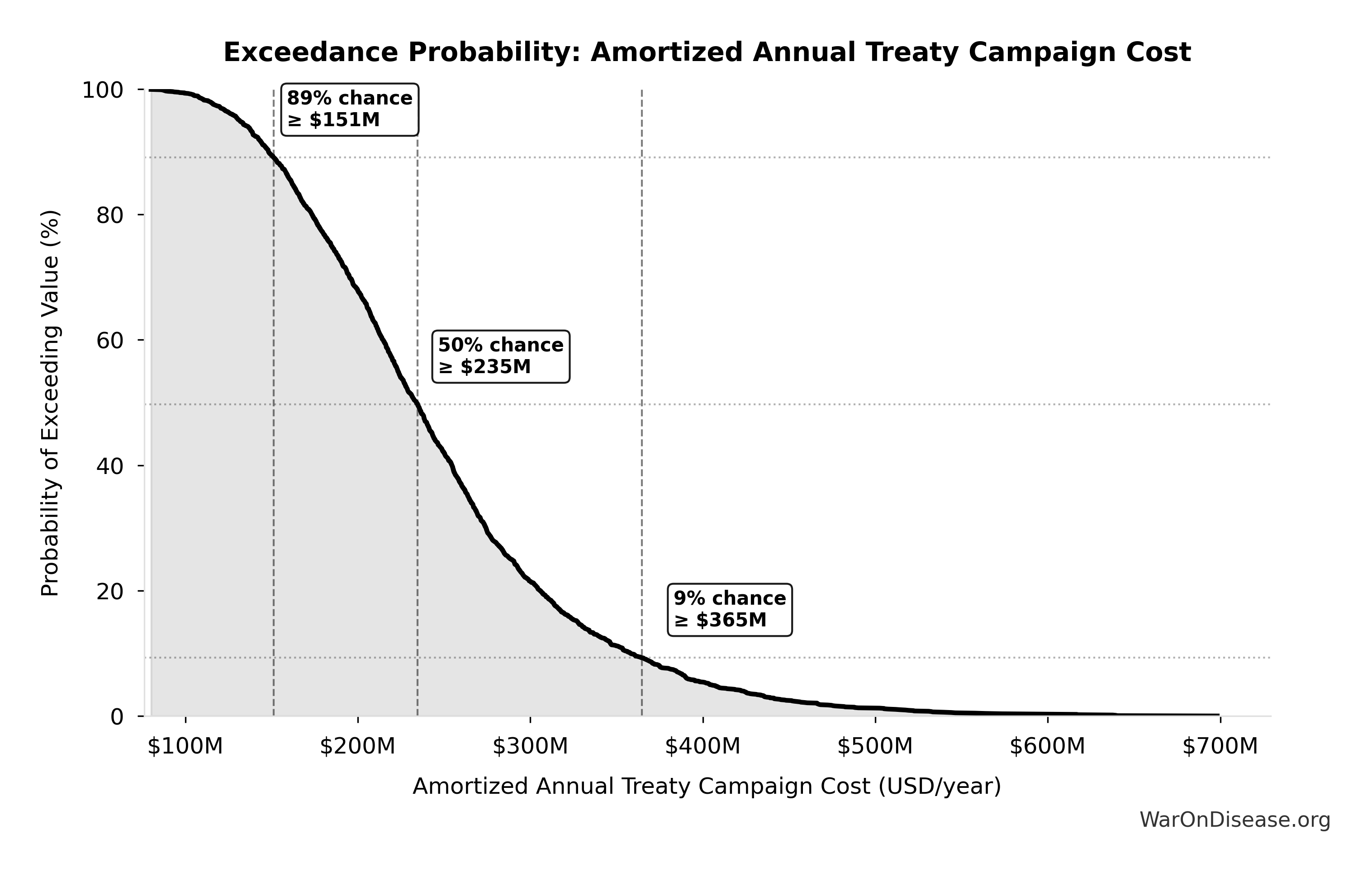
Sensitivity Indices for Expected Cost per DALY (Risk-Adjusted)
Regression-based sensitivity showing which inputs explain the most variance in the output.
| Input Parameter | Sensitivity Coefficient | Interpretation |
|---|---|---|
| Cost per DALY Averted (Elimination of Efficacy Lag Plus Earlier Treatment Discovery from Increased Trial Throughput) (USD/DALY) | 0.5667 | Strong driver |
| Political Success Probability (rate) | -0.4439 | Moderate driver |
Interpretation: Standardized coefficients show the change in output (in SD units) per 1 SD change in input. Values near ±1 indicate strong influence; values exceeding ±1 may occur with correlated inputs.
Monte Carlo Distribution
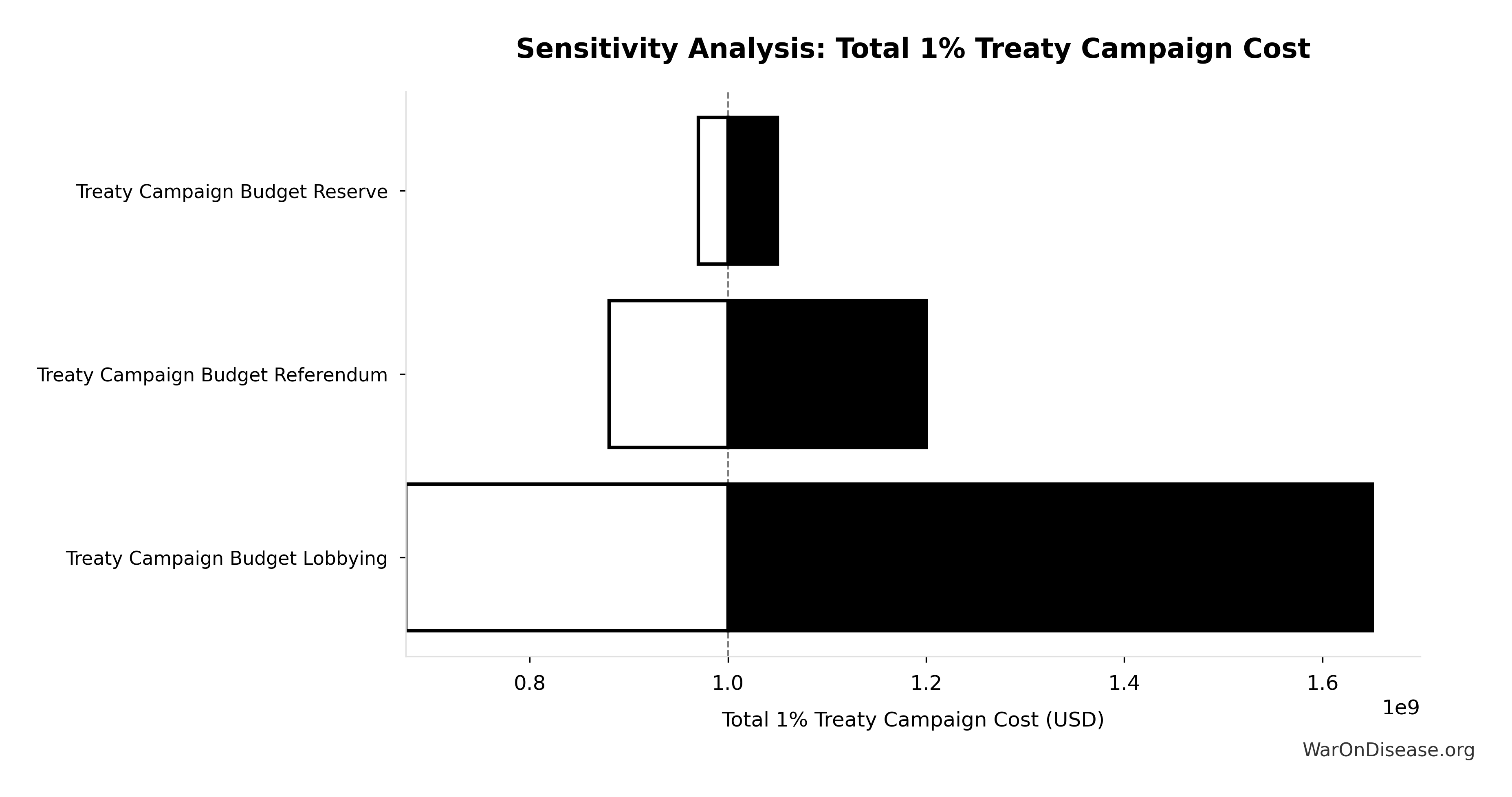
Simulation Results Summary: Expected Cost per DALY (Risk-Adjusted)
| Statistic | Value |
|---|---|
| Baseline (deterministic) | $0.177 |
| Mean (expected value) | $1.06 |
| Median (50th percentile) | $0.778 |
| Standard Deviation | $1.12 |
| 90% Range (5th-95th percentile) | [$0.029, $3.2] |
The histogram shows the distribution of Expected Cost per DALY (Risk-Adjusted) across 10,000 Monte Carlo simulations. The CDF (right) shows the probability of the outcome exceeding any given value, which is useful for risk assessment.
Exceedance Probability
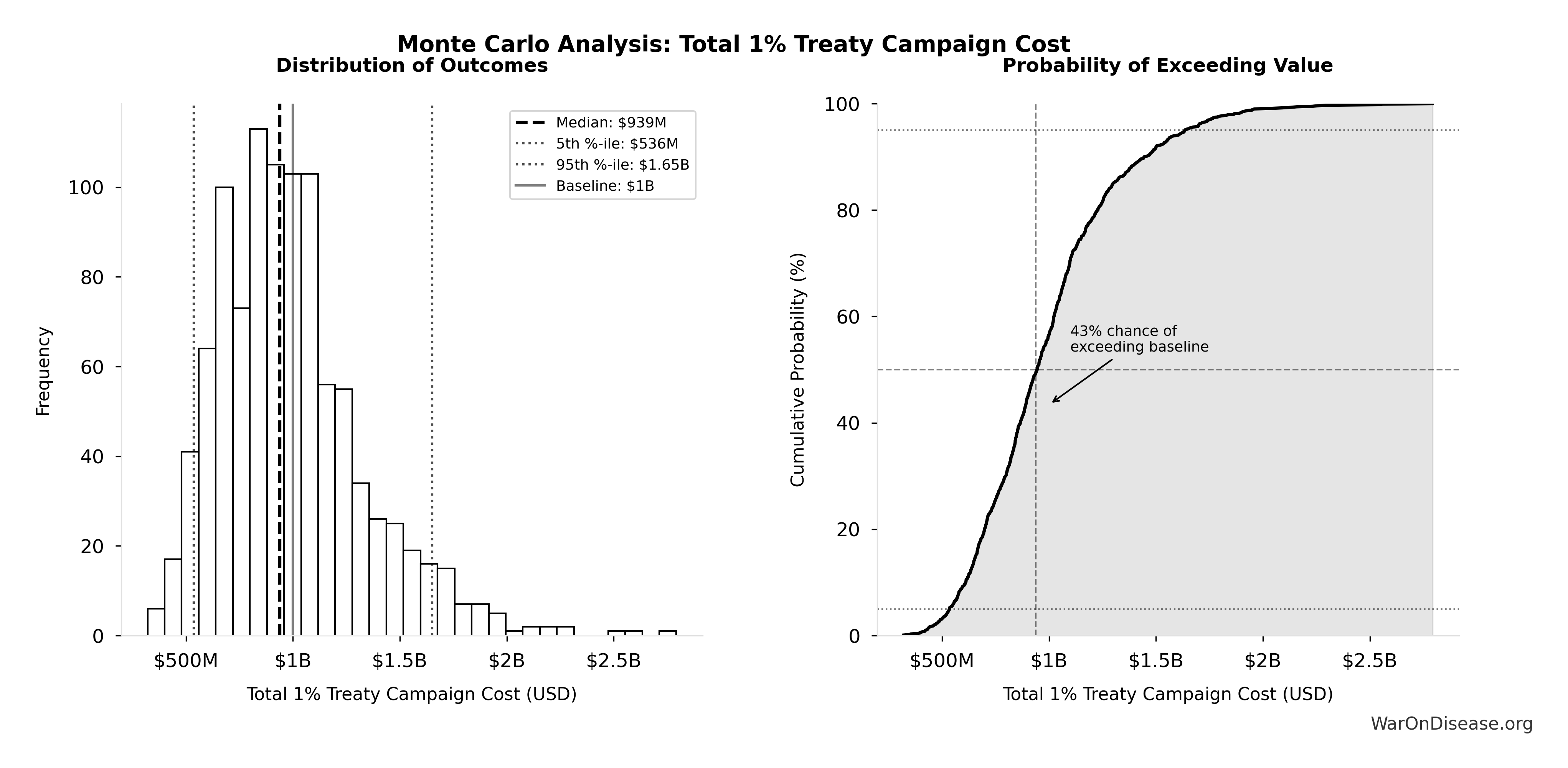
This exceedance probability chart shows the likelihood that Expected Cost per DALY (Risk-Adjusted) will exceed any given threshold. Higher curves indicate more favorable outcomes with greater certainty.
Expected Treaty ROI (Risk-Adjusted): 848k:1
Note📊 Details
Expected ROI for 1% treaty accounting for political success probability uncertainty. Monte Carlo samples POLITICAL_SUCCESS_PROBABILITY from beta(0.1%, 10%) distribution to generate full expected value distribution. Central value uses 1% probability.
Inputs:
- Treaty ROI - Elimination of Efficacy Lag Plus Earlier Treatment Discovery from Increased Trial Throughput 🔢: 84.8M:1
- Political Success Probability 📊: 1% (95% CI: 0.1% - 10%)
\[ \begin{gathered} E[ROI_{max}] \\ = ROI_{max} \times P_{success} \\ = 84.8M \times 1\% \\ = 848{,}000 \end{gathered} \] where: \[ \begin{gathered} ROI_{max} \\ = \frac{Value_{max}}{Cost_{campaign}} \\ = \frac{\$84800T}{\$1B} \\ = 84.8M \end{gathered} \] where: \[ \begin{gathered} Value_{max} \\ = DALYs_{max} \times Value_{QALY} \\ = 565B \times \$150K \\ = \$84800T \end{gathered} \] where: \[ \begin{gathered} DALYs_{max} \\ = DALYs_{global,ann} \times Pct_{avoid,DALY} \times T_{accel,max} \\ = 2.88B \times 92.6\% \times 212 \\ = 565B \end{gathered} \] where: \[ T_{accel,max} = T_{accel} + T_{lag} = 204 + 8.2 = 212 \] where: \[ \begin{gathered} T_{accel} \\ = T_{first,SQ} \times \left(1 - \frac{1}{k_{capacity}}\right) \\ = 222 \times \left(1 - \frac{1}{12.3}\right) \\ = 204 \end{gathered} \] where: \[ \begin{gathered} T_{first,SQ} \\ = T_{queue,SQ} \times 0.5 \\ = 443 \times 0.5 \\ = 222 \end{gathered} \] where: \[ \begin{gathered} T_{queue,SQ} \\ = \frac{N_{untreated}}{Treatments_{new,ann}} \\ = \frac{6{,}650}{15} \\ = 443 \end{gathered} \] where: \[ \begin{gathered} N_{untreated} \\ = N_{rare} \times 0.95 \\ = 7{,}000 \times 0.95 \\ = 6{,}650 \end{gathered} \] where: \[ \begin{gathered} k_{capacity} \\ = \frac{N_{fundable,dFDA}}{Slots_{curr}} \\ = \frac{23.4M}{1.9M} \\ = 12.3 \end{gathered} \] where: \[ \begin{gathered} N_{fundable,dFDA} \\ = \frac{Subsidies_{dFDA,ann}}{Cost_{pragmatic,pt}} \\ = \frac{\$21.8B}{\$929} \\ = 23.4M \end{gathered} \] where: \[ \begin{gathered} Subsidies_{dFDA,ann} \\ = Funding_{dFDA,ann} - OPEX_{dFDA} \\ = \$21.8B - \$40M \\ = \$21.8B \end{gathered} \] where: \[ \begin{gathered} OPEX_{dFDA} \\ = Cost_{platform} + Cost_{staff} + Cost_{infra} \\ + Cost_{regulatory} + Cost_{community} \\ = \$15M + \$10M + \$8M + \$5M + \$2M \\ = \$40M \end{gathered} \] where: \[ \begin{gathered} Cost_{campaign} \\ = Budget_{viral,base} + Budget_{lobby,treaty} \\ + Budget_{reserve} \\ = \$250M + \$650M + \$100M \\ = \$1B \end{gathered} \] Methodology: Direct Calculation
? Low confidence
Sensitivity Analysis
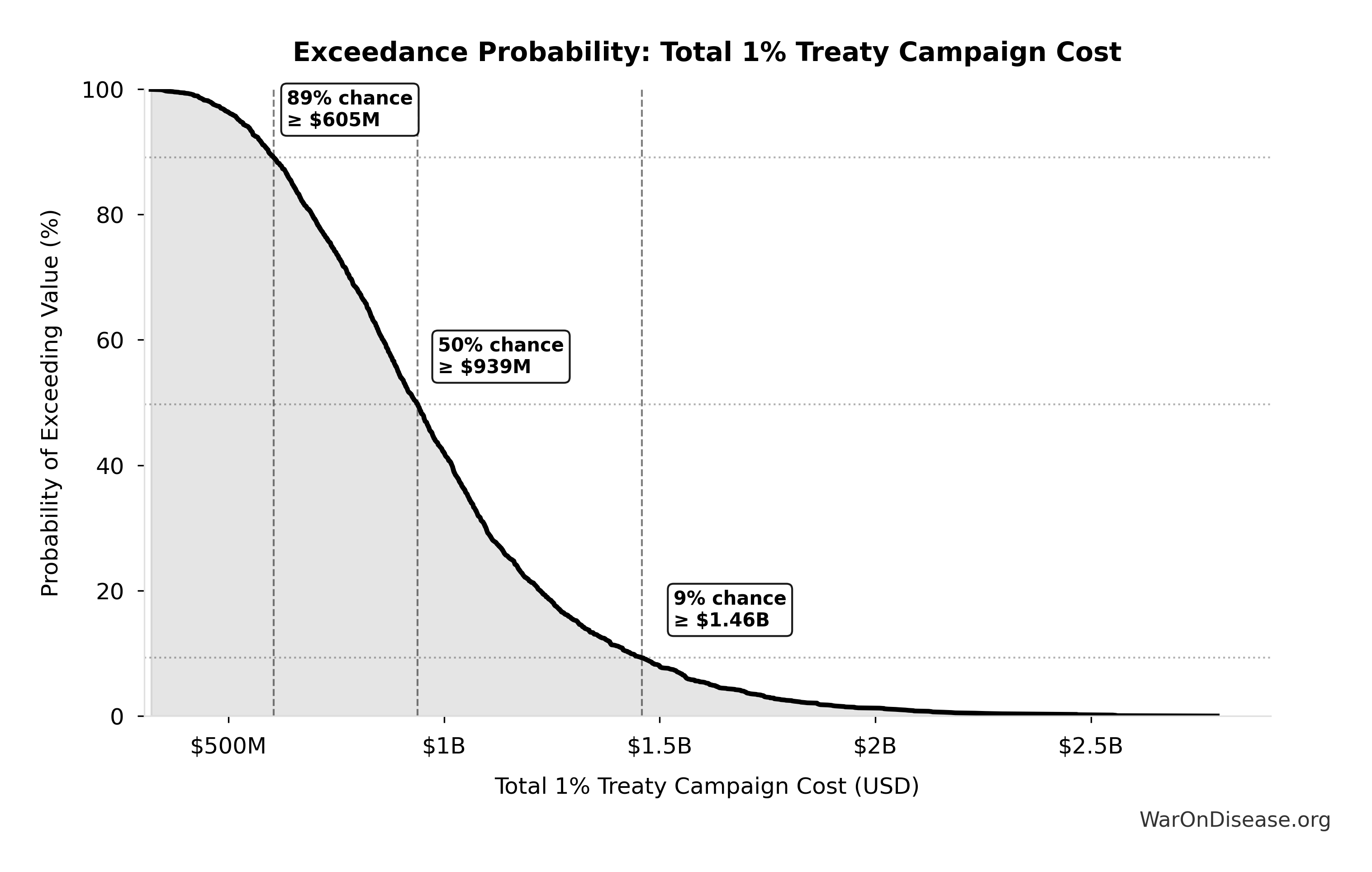
Sensitivity Indices for Expected Treaty ROI (Risk-Adjusted)
Regression-based sensitivity showing which inputs explain the most variance in the output.
| Input Parameter | Sensitivity Coefficient | Interpretation |
|---|---|---|
| Political Success Probability (rate) | 0.9453 | Strong driver |
| Treaty ROI - Elimination of Efficacy Lag Plus Earlier Treatment Discovery from Increased Trial Throughput (ratio) | 0.1601 | Weak driver |
Interpretation: Standardized coefficients show the change in output (in SD units) per 1 SD change in input. Values near ±1 indicate strong influence; values exceeding ±1 may occur with correlated inputs.
Monte Carlo Distribution
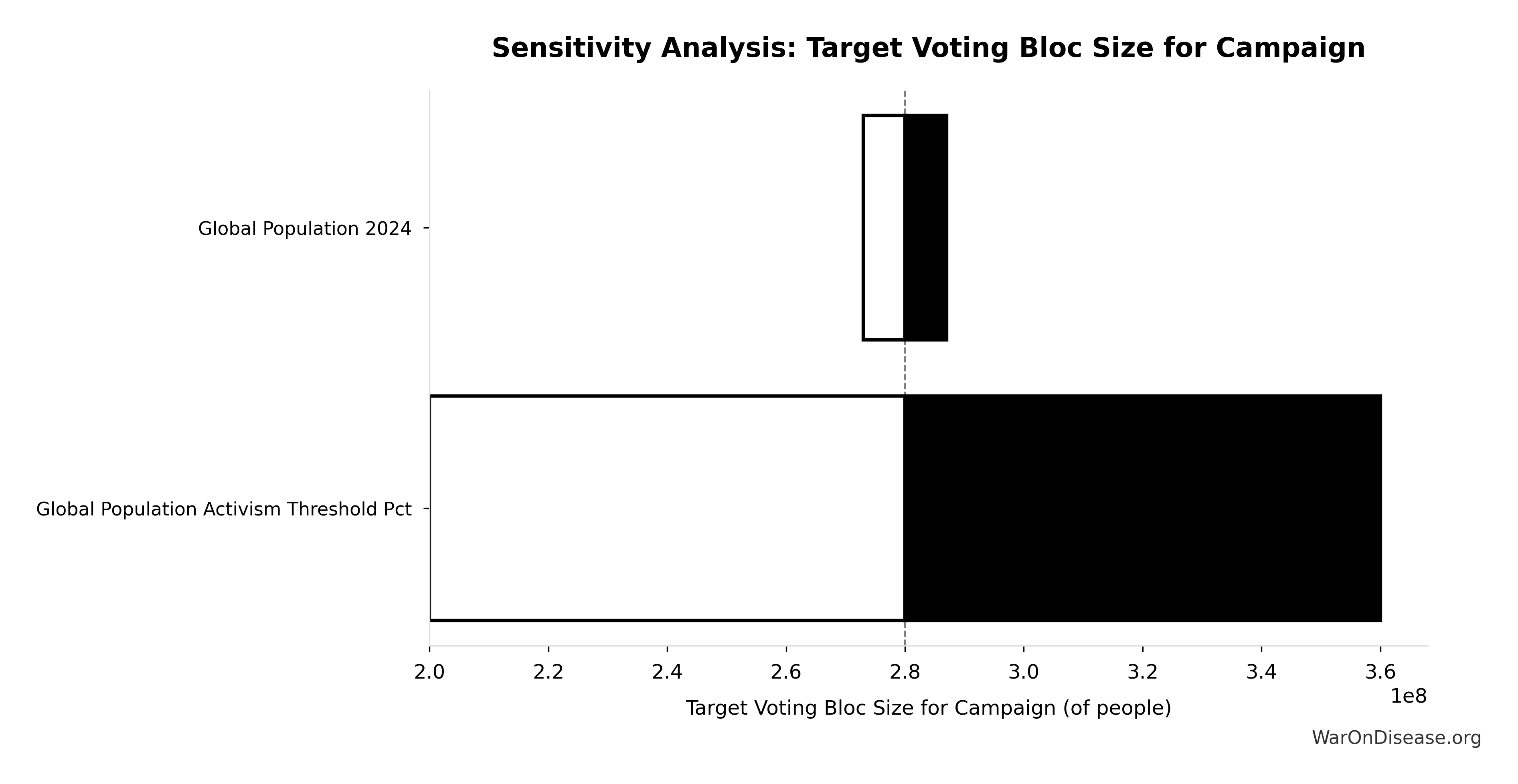
Simulation Results Summary: Expected Treaty ROI (Risk-Adjusted)
| Statistic | Value |
|---|---|
| Baseline (deterministic) | 848k:1 |
| Mean (expected value) | 963k:1 |
| Median (50th percentile) | 154k:1 |
| Standard Deviation | 1.80M:1 |
| 90% Range (5th-95th percentile) | [58.0k:1, 4.76M:1] |
The histogram shows the distribution of Expected Treaty ROI (Risk-Adjusted) across 10,000 Monte Carlo simulations. The CDF (right) shows the probability of the outcome exceeding any given value, which is useful for risk assessment.
Exceedance Probability
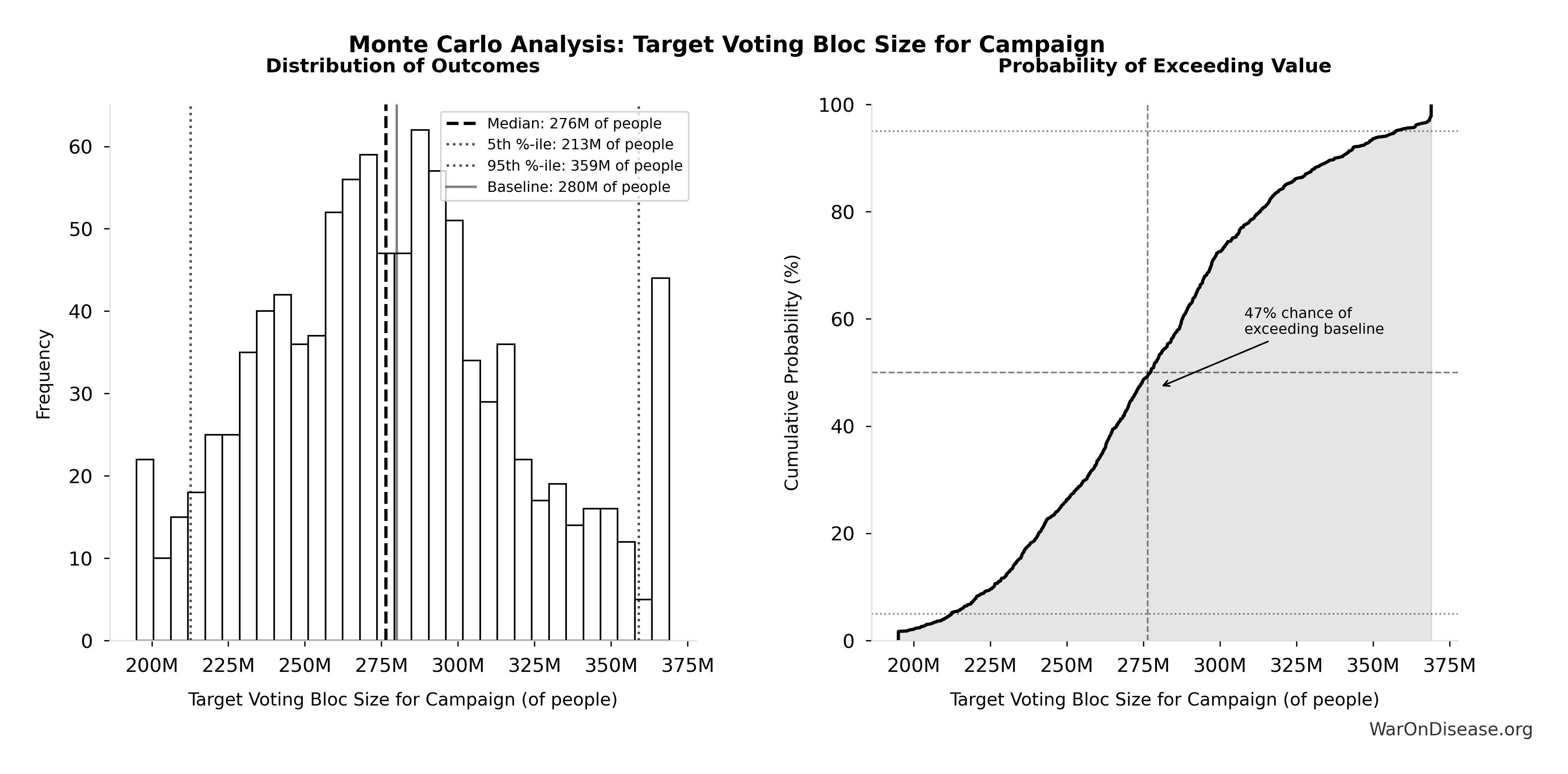
This exceedance probability chart shows the likelihood that Expected Treaty ROI (Risk-Adjusted) will exceed any given threshold. Higher curves indicate more favorable outcomes with greater certainty.
Expected Cost-Effectiveness vs Bed Nets Multiplier: 503x
Note📊 Details
Expected value multiplier vs bed nets (accounts for political uncertainty at 1% success rate)
Inputs:
- Bed Nets Cost per DALY 📊: $89 (95% CI: $78 - $100)
- Expected Cost per DALY (Risk-Adjusted) 🔢: $0.177
\[ \begin{gathered} E[k_{nets}] \\ = \frac{Cost_{nets}}{E[Cost_{DALY}]} \\ = \frac{\$89}{\$0.177} \\ = 503 \end{gathered} \] where: \[ \begin{gathered} E[Cost_{DALY}] \\ = \frac{Cost_{treaty,DALY}}{P_{success}} \\ = \frac{\$0.00177}{1\%} \\ = \$0.177 \end{gathered} \] where: \[ \begin{gathered} Cost_{treaty,DALY} \\ = \frac{Cost_{campaign}}{DALYs_{max}} \\ = \frac{\$1B}{565B} \\ = \$0.00177 \end{gathered} \] where: \[ \begin{gathered} Cost_{campaign} \\ = Budget_{viral,base} + Budget_{lobby,treaty} \\ + Budget_{reserve} \\ = \$250M + \$650M + \$100M \\ = \$1B \end{gathered} \] where: \[ \begin{gathered} DALYs_{max} \\ = DALYs_{global,ann} \times Pct_{avoid,DALY} \times T_{accel,max} \\ = 2.88B \times 92.6\% \times 212 \\ = 565B \end{gathered} \] where: \[ T_{accel,max} = T_{accel} + T_{lag} = 204 + 8.2 = 212 \] where: \[ \begin{gathered} T_{accel} \\ = T_{first,SQ} \times \left(1 - \frac{1}{k_{capacity}}\right) \\ = 222 \times \left(1 - \frac{1}{12.3}\right) \\ = 204 \end{gathered} \] where: \[ \begin{gathered} T_{first,SQ} \\ = T_{queue,SQ} \times 0.5 \\ = 443 \times 0.5 \\ = 222 \end{gathered} \] where: \[ \begin{gathered} T_{queue,SQ} \\ = \frac{N_{untreated}}{Treatments_{new,ann}} \\ = \frac{6{,}650}{15} \\ = 443 \end{gathered} \] where: \[ \begin{gathered} N_{untreated} \\ = N_{rare} \times 0.95 \\ = 7{,}000 \times 0.95 \\ = 6{,}650 \end{gathered} \] where: \[ \begin{gathered} k_{capacity} \\ = \frac{N_{fundable,dFDA}}{Slots_{curr}} \\ = \frac{23.4M}{1.9M} \\ = 12.3 \end{gathered} \] where: \[ \begin{gathered} N_{fundable,dFDA} \\ = \frac{Subsidies_{dFDA,ann}}{Cost_{pragmatic,pt}} \\ = \frac{\$21.8B}{\$929} \\ = 23.4M \end{gathered} \] where: \[ \begin{gathered} Subsidies_{dFDA,ann} \\ = Funding_{dFDA,ann} - OPEX_{dFDA} \\ = \$21.8B - \$40M \\ = \$21.8B \end{gathered} \] where: \[ \begin{gathered} OPEX_{dFDA} \\ = Cost_{platform} + Cost_{staff} + Cost_{infra} \\ + Cost_{regulatory} + Cost_{community} \\ = \$15M + \$10M + \$8M + \$5M + \$2M \\ = \$40M \end{gathered} \] ? Low confidence
Sensitivity Analysis
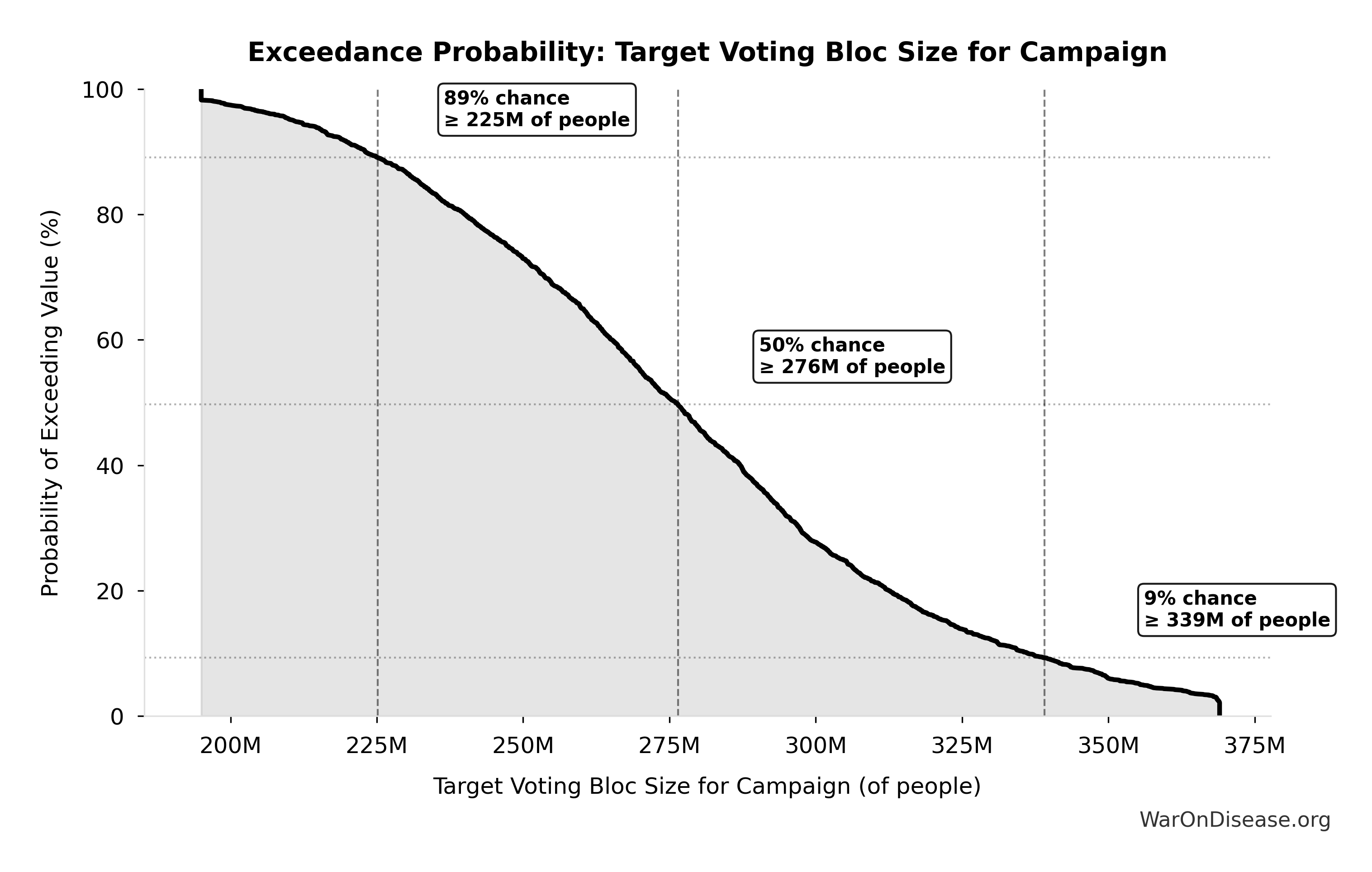
Sensitivity Indices for Expected Cost-Effectiveness vs Bed Nets Multiplier
Regression-based sensitivity showing which inputs explain the most variance in the output.
| Input Parameter | Sensitivity Coefficient | Interpretation |
|---|---|---|
| Expected Cost per DALY (Risk-Adjusted) (USD/DALY) | -0.4157 | Moderate driver |
| Bed Nets Cost per DALY (USD/DALY) | 0.0040 | Minimal effect |
Interpretation: Standardized coefficients show the change in output (in SD units) per 1 SD change in input. Values near ±1 indicate strong influence; values exceeding ±1 may occur with correlated inputs.
Monte Carlo Distribution
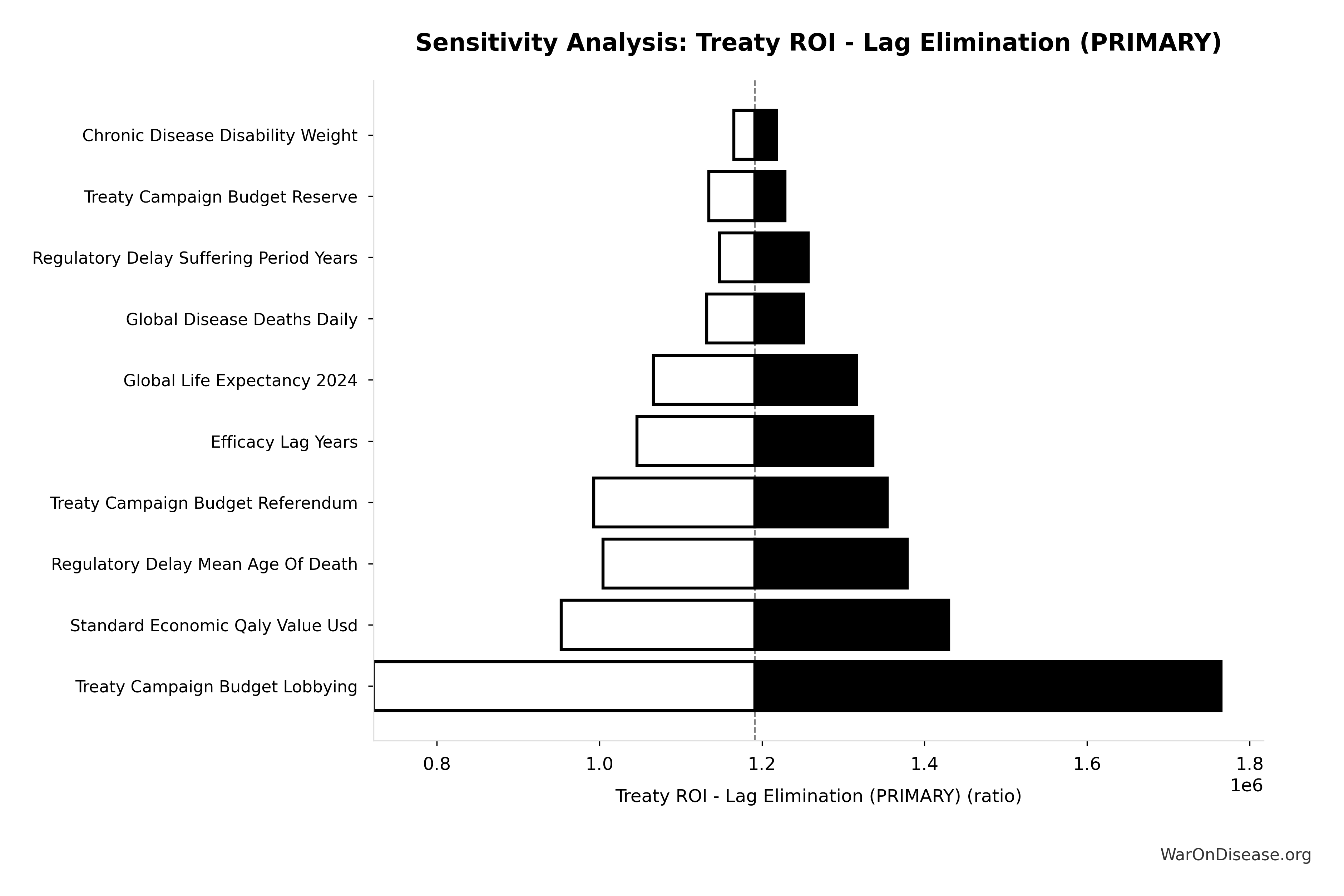
Simulation Results Summary: Expected Cost-Effectiveness vs Bed Nets Multiplier
| Statistic | Value |
|---|---|
| Baseline (deterministic) | 503x |
| Mean (expected value) | 606x |
| Median (50th percentile) | 109x |
| Standard Deviation | 1.2kx |
| 90% Range (5th-95th percentile) | [30x, 3.0kx] |
The histogram shows the distribution of Expected Cost-Effectiveness vs Bed Nets Multiplier across 10,000 Monte Carlo simulations. The CDF (right) shows the probability of the outcome exceeding any given value, which is useful for risk assessment.
Exceedance Probability
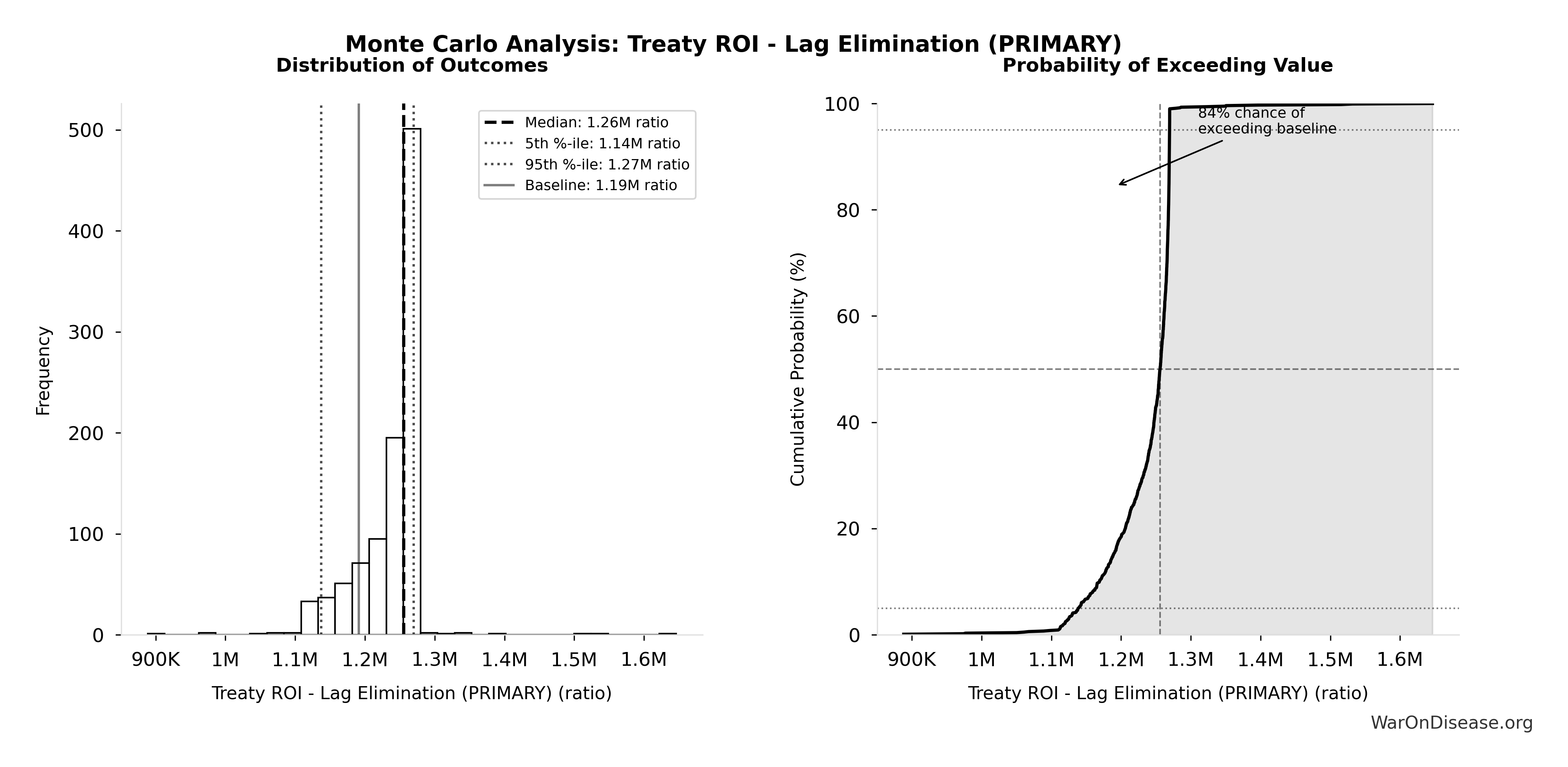
This exceedance probability chart shows the likelihood that Expected Cost-Effectiveness vs Bed Nets Multiplier will exceed any given threshold. Higher curves indicate more favorable outcomes with greater certainty.
1% treaty Basic Annual Benefits (Peace + R&D Savings): $172B
Note📊 Details
Basic annual benefits: peace dividend + Decentralized Framework for Drug Assessment R&D savings only (2 of 8 benefit categories, excludes regulatory delay value)
Inputs:
- Annual Peace Dividend from 1% Reduction in Total War Costs 🔢: $114B
- Decentralized Framework for Drug Assessment Annual Benefit: R&D Savings 🔢: $58.6B
\[ \begin{gathered} Benefit_{peace+RD} \\ = Benefit_{peace,soc} + Benefit_{RD,ann} \\ = \$114B + \$58.6B \\ = \$172B \end{gathered} \] where: \[ \begin{gathered} Benefit_{peace,soc} \\ = Cost_{war,total} \times Reduce_{treaty} \\ = \$11.4T \times 1\% \\ = \$114B \end{gathered} \] where: \[ \begin{gathered} Cost_{war,total} \\ = Cost_{war,direct} + Cost_{war,indirect} \\ = \$7.66T + \$3.7T \\ = \$11.4T \end{gathered} \] where: \[ \begin{gathered} Cost_{war,direct} \\ = Loss_{life,conflict} + Damage_{infra,total} \\ + Disruption_{trade} + Spending_{mil} \\ = \$2.45T + \$1.88T + \$616B + \$2.72T \\ = \$7.66T \end{gathered} \] where: \[ \begin{gathered} Loss_{life,conflict} \\ = Cost_{combat,human} + Cost_{state,human} \\ + Cost_{terror,human} \\ = \$2.34T + \$27B + \$83B \\ = \$2.45T \end{gathered} \] where: \[ \begin{gathered} Cost_{combat,human} \\ = Deaths_{combat} \times VSL \\ = 234{,}000 \times \$10M \\ = \$2.34T \end{gathered} \] where: \[ \begin{gathered} Cost_{state,human} \\ = Deaths_{state} \times VSL \\ = 2{,}700 \times \$10M \\ = \$27B \end{gathered} \] where: \[ \begin{gathered} Cost_{terror,human} \\ = Deaths_{terror} \times VSL \\ = 8{,}300 \times \$10M \\ = \$83B \end{gathered} \] where: \[ \begin{gathered} Damage_{infra,total} \\ = Damage_{comms} + Damage_{edu} + Damage_{energy} \\ + Damage_{health} + Damage_{transport} + Damage_{water} \\ = \$298B + \$234B + \$422B + \$166B + \$487B + \$268B \\ = \$1.88T \end{gathered} \] where: \[ \begin{gathered} Disruption_{trade} \\ = Disruption_{currency} + Disruption_{energy} \\ + Disruption_{shipping} + Disruption_{supply} \\ = \$57.4B + \$125B + \$247B + \$187B \\ = \$616B \end{gathered} \] where: \[ \begin{gathered} Cost_{war,indirect} \\ = Damage_{env} + Loss_{growth,mil} + Loss_{capital,conflict} \\ + Cost_{psych} + Cost_{refugee} + Cost_{vet} \\ = \$100B + \$2.72T + \$300B + \$232B + \$150B + \$200B \\ = \$3.7T \end{gathered} \] where: \[ \begin{gathered} Benefit_{RD,ann} \\ = Spending_{trials} \times Reduce_{pct} \\ = \$60B \times 97.7\% \\ = \$58.6B \end{gathered} \] where: \[ \begin{gathered} Reduce_{pct} \\ = 1 - \frac{Cost_{pragmatic,pt}}{Cost_{P3,pt}} \\ = 1 - \frac{\$929}{\$41K} \\ = 97.7\% \end{gathered} \] ✓ High confidence
Sensitivity Analysis
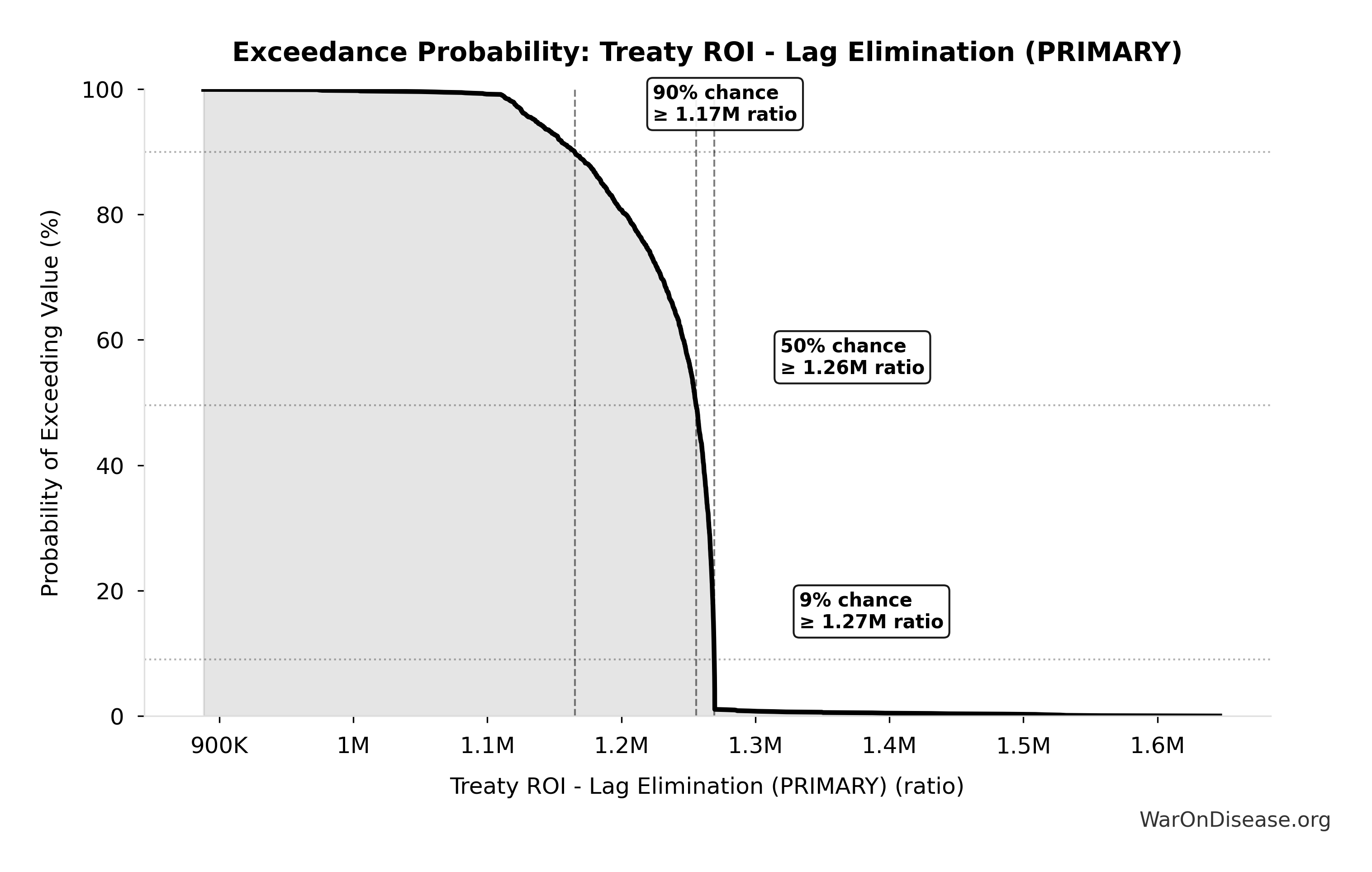
Sensitivity Indices for 1% treaty Basic Annual Benefits (Peace + R&D Savings)
Regression-based sensitivity showing which inputs explain the most variance in the output.
| Input Parameter | Sensitivity Coefficient | Interpretation |
|---|---|---|
| Annual Peace Dividend from 1% Reduction in Total War Costs (USD/year) | 0.6828 | Strong driver |
| Decentralized Framework for Drug Assessment Annual Benefit: R&D Savings (USD/year) | 0.3457 | Moderate driver |
Interpretation: Standardized coefficients show the change in output (in SD units) per 1 SD change in input. Values near ±1 indicate strong influence; values exceeding ±1 may occur with correlated inputs.
Monte Carlo Distribution
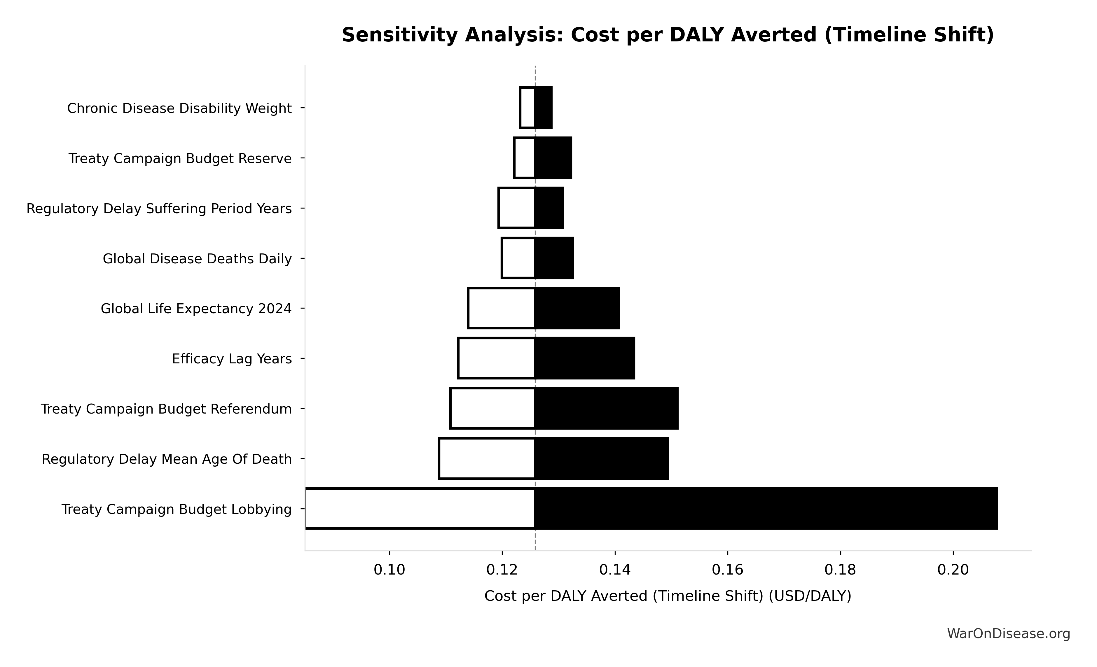
Simulation Results Summary: 1% treaty Basic Annual Benefits (Peace + R&D Savings)
| Statistic | Value |
|---|---|
| Baseline (deterministic) | $172B |
| Mean (expected value) | $172B |
| Median (50th percentile) | $170B |
| Standard Deviation | $22.2B |
| 90% Range (5th-95th percentile) | [$140B, $213B] |
The histogram shows the distribution of 1% treaty Basic Annual Benefits (Peace + R&D Savings) across 10,000 Monte Carlo simulations. The CDF (right) shows the probability of the outcome exceeding any given value, which is useful for risk assessment.
Exceedance Probability
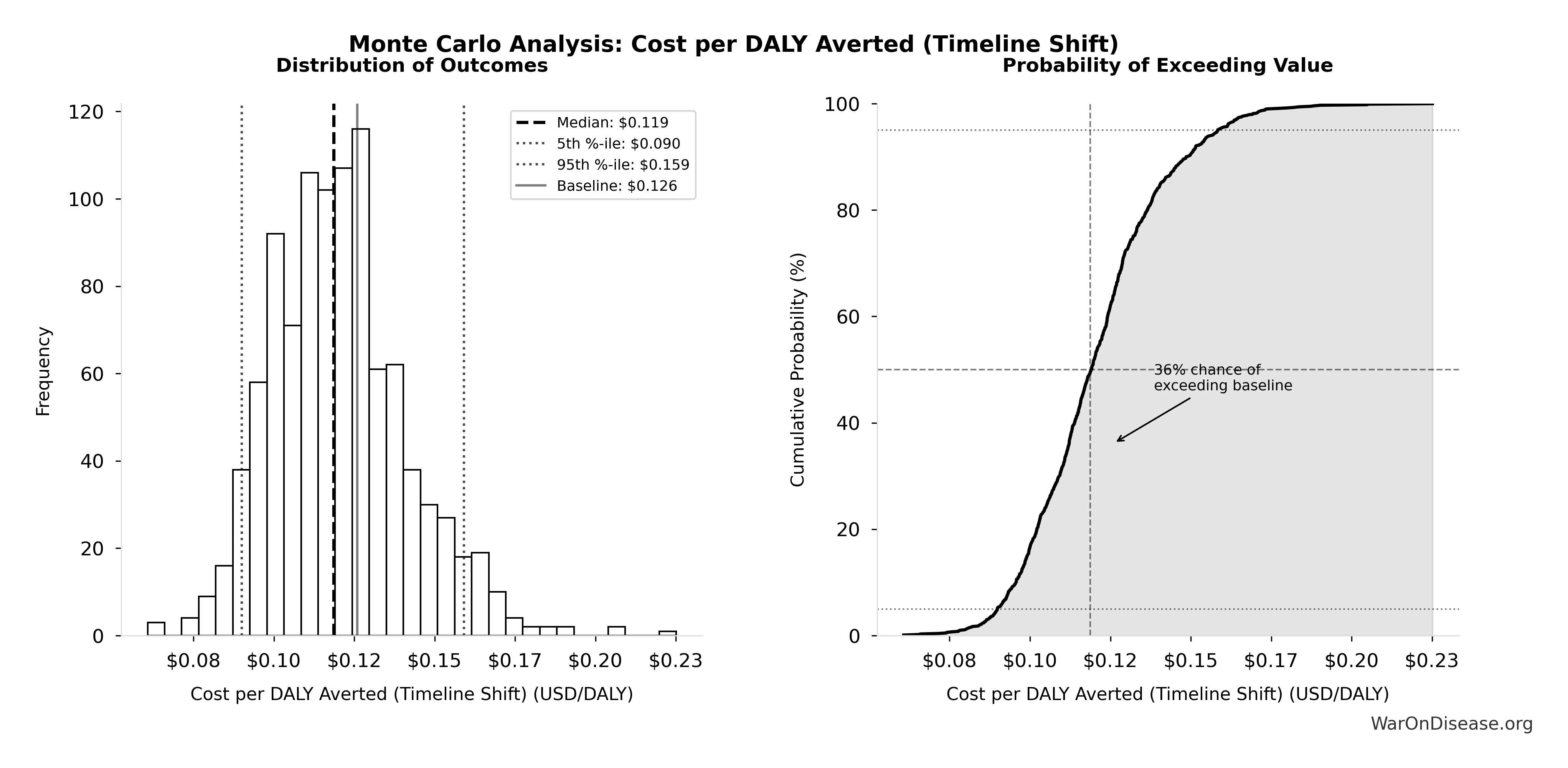
This exceedance probability chart shows the likelihood that 1% treaty Basic Annual Benefits (Peace + R&D Savings) will exceed any given threshold. Higher curves indicate more favorable outcomes with greater certainty.
Treaty ROI - Elimination of Efficacy Lag Plus Earlier Treatment Discovery from Increased Trial Throughput: 84.8M:1
Note📊 Details
Treaty ROI from elimination of efficacy lag plus earlier treatment discovery from increased trial throughput. Total one-time benefit divided by campaign cost. This is the primary ROI estimate for total health benefits.
Inputs:
- Total Economic Benefit from Elimination of Efficacy Lag Plus Earlier Treatment Discovery from Higher Trial Throughput 🔢: $84.8 quadrillion
- Total 1% Treaty Campaign Cost 🔢: $1B
\[ \begin{gathered} ROI_{max} \\ = \frac{Value_{max}}{Cost_{campaign}} \\ = \frac{\$84800T}{\$1B} \\ = 84.8M \end{gathered} \] where: \[ \begin{gathered} Value_{max} \\ = DALYs_{max} \times Value_{QALY} \\ = 565B \times \$150K \\ = \$84800T \end{gathered} \] where: \[ \begin{gathered} DALYs_{max} \\ = DALYs_{global,ann} \times Pct_{avoid,DALY} \times T_{accel,max} \\ = 2.88B \times 92.6\% \times 212 \\ = 565B \end{gathered} \] where: \[ T_{accel,max} = T_{accel} + T_{lag} = 204 + 8.2 = 212 \] where: \[ \begin{gathered} T_{accel} \\ = T_{first,SQ} \times \left(1 - \frac{1}{k_{capacity}}\right) \\ = 222 \times \left(1 - \frac{1}{12.3}\right) \\ = 204 \end{gathered} \] where: \[ \begin{gathered} T_{first,SQ} \\ = T_{queue,SQ} \times 0.5 \\ = 443 \times 0.5 \\ = 222 \end{gathered} \] where: \[ \begin{gathered} T_{queue,SQ} \\ = \frac{N_{untreated}}{Treatments_{new,ann}} \\ = \frac{6{,}650}{15} \\ = 443 \end{gathered} \] where: \[ \begin{gathered} N_{untreated} \\ = N_{rare} \times 0.95 \\ = 7{,}000 \times 0.95 \\ = 6{,}650 \end{gathered} \] where: \[ \begin{gathered} k_{capacity} \\ = \frac{N_{fundable,dFDA}}{Slots_{curr}} \\ = \frac{23.4M}{1.9M} \\ = 12.3 \end{gathered} \] where: \[ \begin{gathered} N_{fundable,dFDA} \\ = \frac{Subsidies_{dFDA,ann}}{Cost_{pragmatic,pt}} \\ = \frac{\$21.8B}{\$929} \\ = 23.4M \end{gathered} \] where: \[ \begin{gathered} Subsidies_{dFDA,ann} \\ = Funding_{dFDA,ann} - OPEX_{dFDA} \\ = \$21.8B - \$40M \\ = \$21.8B \end{gathered} \] where: \[ \begin{gathered} OPEX_{dFDA} \\ = Cost_{platform} + Cost_{staff} + Cost_{infra} \\ + Cost_{regulatory} + Cost_{community} \\ = \$15M + \$10M + \$8M + \$5M + \$2M \\ = \$40M \end{gathered} \] where: \[ \begin{gathered} Cost_{campaign} \\ = Budget_{viral,base} + Budget_{lobby,treaty} \\ + Budget_{reserve} \\ = \$250M + \$650M + \$100M \\ = \$1B \end{gathered} \] ~ Medium confidence
Sensitivity Analysis
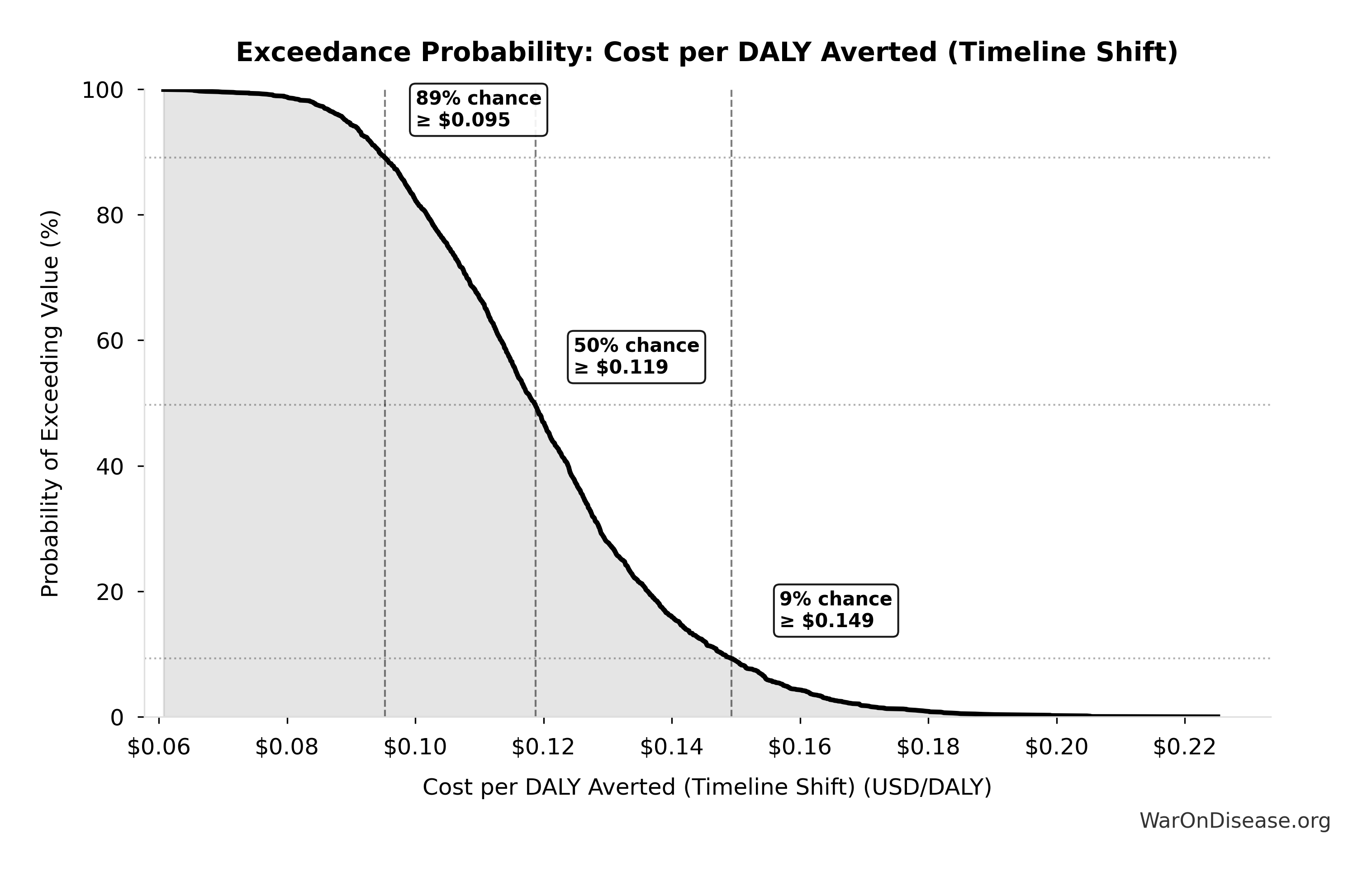
Sensitivity Indices for Treaty ROI - Elimination of Efficacy Lag Plus Earlier Treatment Discovery from Increased Trial Throughput
Regression-based sensitivity showing which inputs explain the most variance in the output.
| Input Parameter | Sensitivity Coefficient | Interpretation |
|---|---|---|
| Total 1% Treaty Campaign Cost (USD) | -0.7930 | Strong driver |
| Total Economic Benefit from Elimination of Efficacy Lag Plus Earlier Treatment Discovery from Higher Trial Throughput (USD) | 0.3364 | Moderate driver |
Interpretation: Standardized coefficients show the change in output (in SD units) per 1 SD change in input. Values near ±1 indicate strong influence; values exceeding ±1 may occur with correlated inputs.
Monte Carlo Distribution
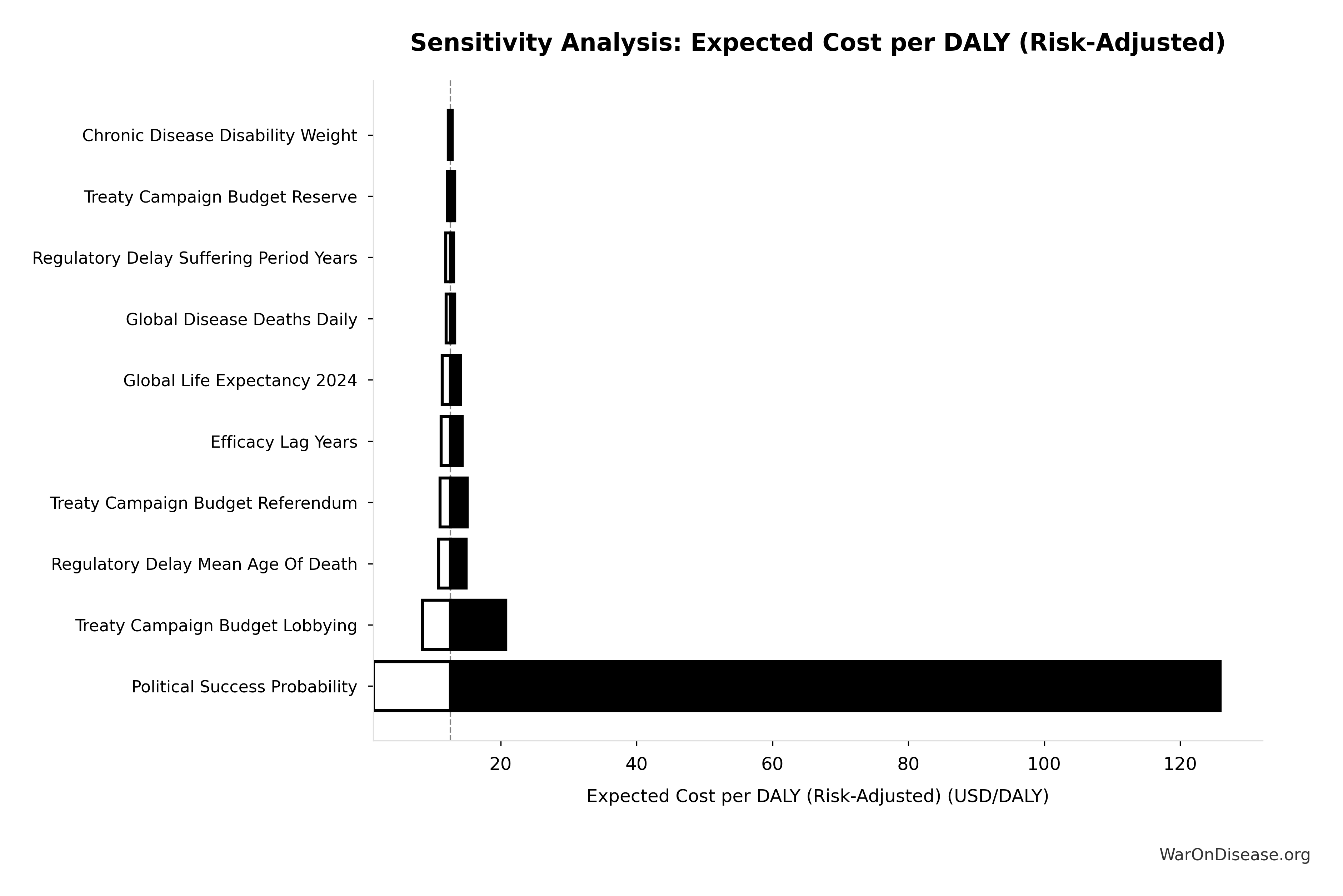
Simulation Results Summary: Treaty ROI - Elimination of Efficacy Lag Plus Earlier Treatment Discovery from Increased Trial Throughput
| Statistic | Value |
|---|---|
| Baseline (deterministic) | 84.8M:1 |
| Mean (expected value) | 95.1M:1 |
| Median (50th percentile) | 96.0M:1 |
| Standard Deviation | 28.1M:1 |
| 90% Range (5th-95th percentile) | [46.6M:1, 144M:1] |
The histogram shows the distribution of Treaty ROI - Elimination of Efficacy Lag Plus Earlier Treatment Discovery from Increased Trial Throughput across 10,000 Monte Carlo simulations. The CDF (right) shows the probability of the outcome exceeding any given value, which is useful for risk assessment.
Exceedance Probability
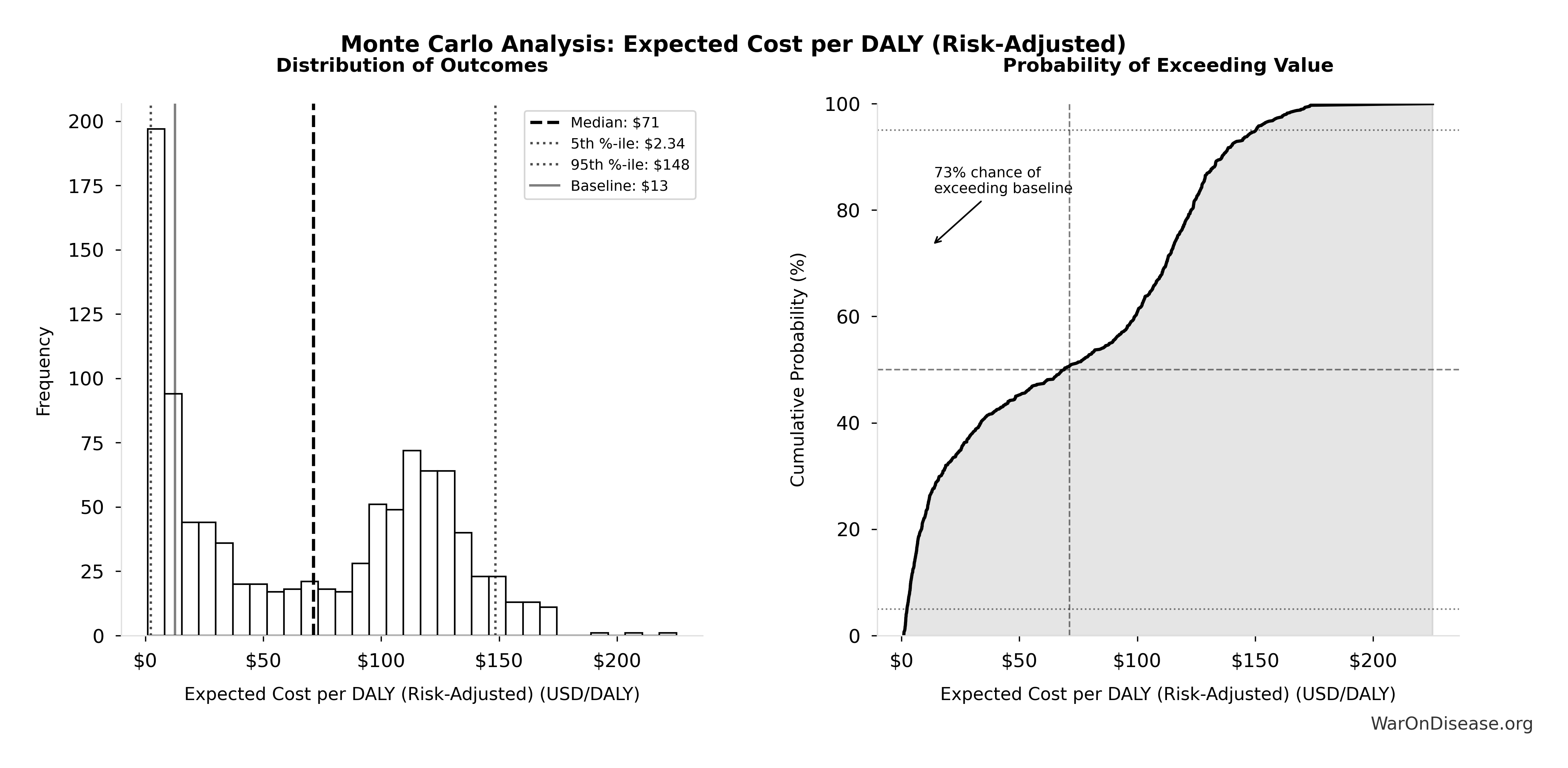
This exceedance probability chart shows the likelihood that Treaty ROI - Elimination of Efficacy Lag Plus Earlier Treatment Discovery from Increased Trial Throughput will exceed any given threshold. Higher curves indicate more favorable outcomes with greater certainty.
Treaty Trajectory Average Income at Year 20: $339K
Note📊 Details
Average income (GDP per capita) at year 20 under the Treaty Trajectory.
Inputs:
- Treaty Trajectory GDP at Year 20 🔢: $3.11 quadrillion
- Global Population 2045 (Projected) 📊: 9.2 billion of people
\[ \bar{y}_{treaty,20} = \frac{GDP_{treaty,20}}{Pop_{2045}} \]
✓ High confidence
Sensitivity Analysis
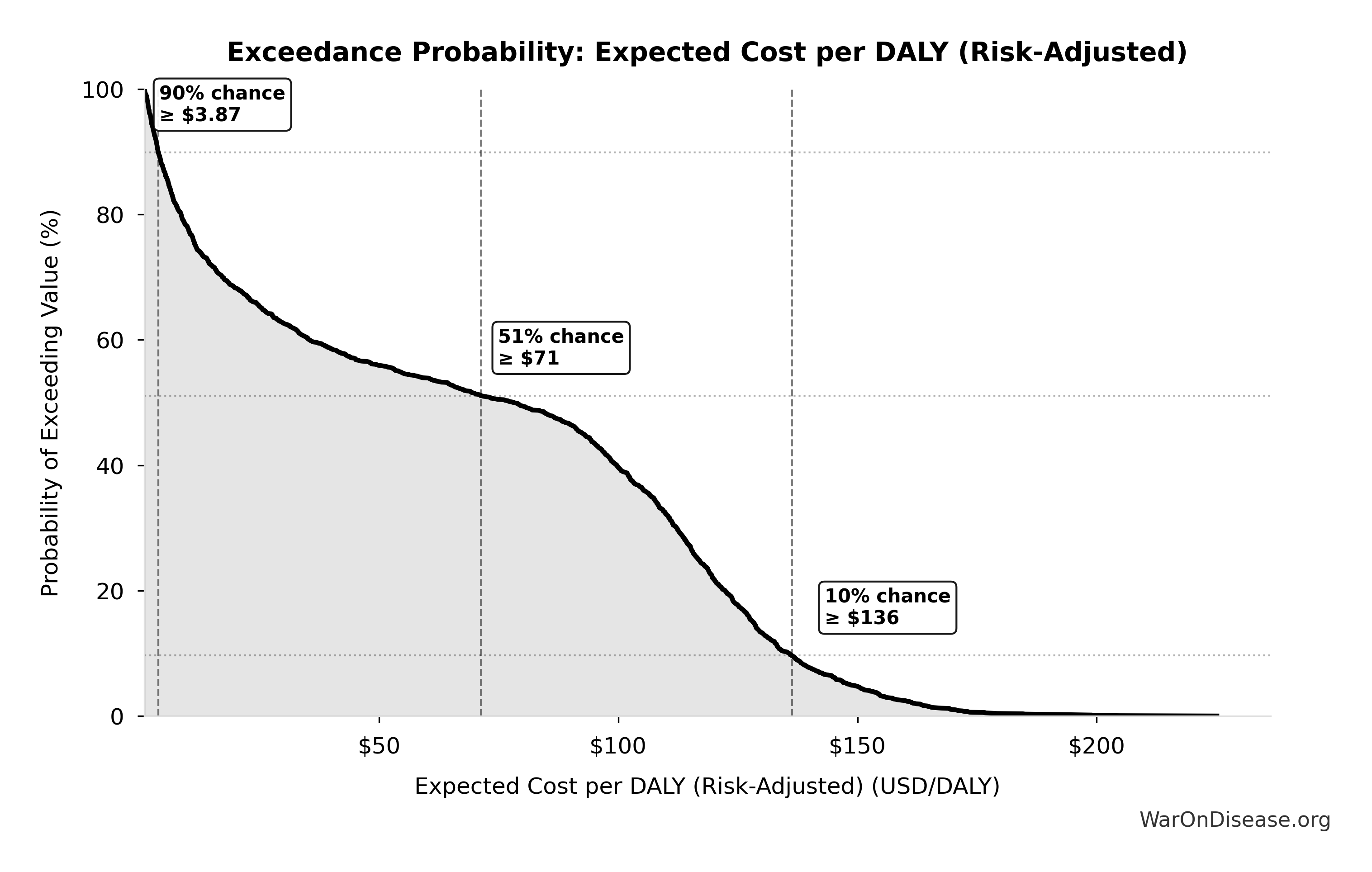
Sensitivity Indices for Treaty Trajectory Average Income at Year 20
Regression-based sensitivity showing which inputs explain the most variance in the output.
| Input Parameter | Sensitivity Coefficient | Interpretation |
|---|---|---|
| Treaty Trajectory GDP at Year 20 (USD) | 1.0000 | Strong driver |
Interpretation: Standardized coefficients show the change in output (in SD units) per 1 SD change in input. Values near ±1 indicate strong influence; values exceeding ±1 may occur with correlated inputs.
Monte Carlo Distribution
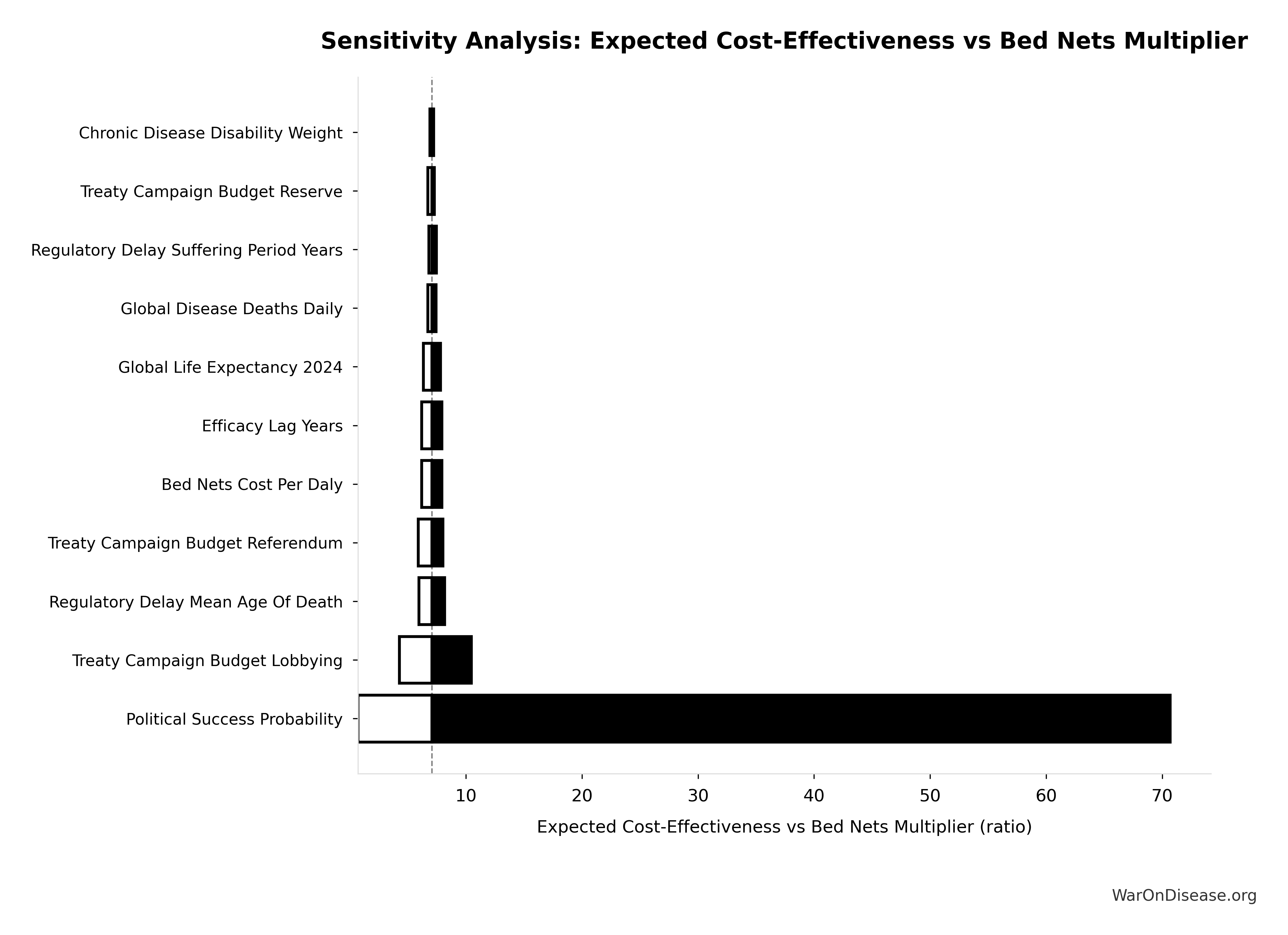
Simulation Results Summary: Treaty Trajectory Average Income at Year 20
| Statistic | Value |
|---|---|
| Baseline (deterministic) | $339K |
| Mean (expected value) | $462K |
| Median (50th percentile) | $335K |
| Standard Deviation | $384K |
| 90% Range (5th-95th percentile) | [$106K, $1.33M] |
The histogram shows the distribution of Treaty Trajectory Average Income at Year 20 across 10,000 Monte Carlo simulations. The CDF (right) shows the probability of the outcome exceeding any given value, which is useful for risk assessment.
Exceedance Probability
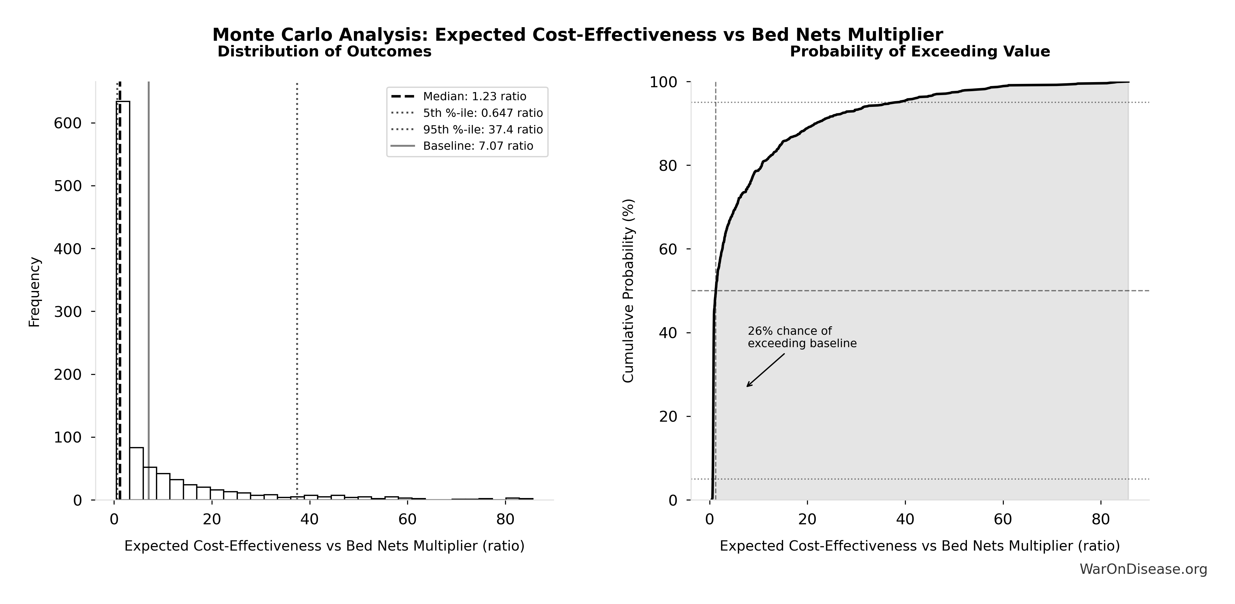
This exceedance probability chart shows the likelihood that Treaty Trajectory Average Income at Year 20 will exceed any given threshold. Higher curves indicate more favorable outcomes with greater certainty.
Treaty Trajectory vs Current Trajectory GDP Multiplier (Year 20): 16.5x
Note📊 Details
Treaty Trajectory GDP at year 20 as a multiple of current trajectory GDP at year 20.
Inputs:
- Treaty Trajectory GDP at Year 20 🔢: $3.11 quadrillion
- Current Trajectory GDP at Year 20 🔢: $188T
\[ \begin{gathered} k_{treaty:base,20} \\ = \frac{GDP_{treaty,20}}{GDP_{base,20}} \\ = \frac{\$3110T}{\$188T} \\ = 16.5 \end{gathered} \] where: \[ \begin{gathered} GDP_{treaty,20} \\ = GDP_0(1+g_{treaty,ramp})^3(1+g_{treaty,full})^{17} \end{gathered} \] where: \[ s_{mil,max} = Cut_{WW2} = 87.6\% = 87.6\% \] where: \[ \begin{gathered} Cut_{WW2} \\ = 1 - \frac{Spending_{US,1947}}{Spending_{US,1945}} \\ = 1 - \frac{\$176B}{\$1.42T} \\ = 87.6\% \end{gathered} \] where: \[ \begin{gathered} f_{cure,20,wish} \\ = \min\left(1,\frac{Treatments_{new,ann}\cdot k_{capacity,wish}\cdot 20}{D_{untreated}}\right) \end{gathered} \] where: \[ \begin{gathered} k_{capacity} \\ = \frac{N_{fundable,dFDA}}{Slots_{curr}} \\ = \frac{23.4M}{1.9M} \\ = 12.3 \end{gathered} \] where: \[ \begin{gathered} N_{fundable,dFDA} \\ = \frac{Subsidies_{dFDA,ann}}{Cost_{pragmatic,pt}} \\ = \frac{\$21.8B}{\$929} \\ = 23.4M \end{gathered} \] where: \[ \begin{gathered} Subsidies_{dFDA,ann} \\ = Funding_{dFDA,ann} - OPEX_{dFDA} \\ = \$21.8B - \$40M \\ = \$21.8B \end{gathered} \] where: \[ \begin{gathered} OPEX_{dFDA} \\ = Cost_{platform} + Cost_{staff} + Cost_{infra} \\ + Cost_{regulatory} + Cost_{community} \\ = \$15M + \$10M + \$8M + \$5M + \$2M \\ = \$40M \end{gathered} \] where: \[ \begin{gathered} k_{capacity,max} \\ = \frac{N_{willing}}{Slots_{curr}} \\ = \frac{1.08B}{1.9M} \\ = 566 \end{gathered} \] where: \[ \begin{gathered} N_{willing} \\ = N_{patients} \times Pct_{willing} \\ = 2.4B \times 44.8\% \\ = 1.08B \end{gathered} \] where: \[ \begin{gathered} N_{untreated} \\ = N_{rare} \times 0.95 \\ = 7{,}000 \times 0.95 \\ = 6{,}650 \end{gathered} \] where: \[ GDP_{base,20} = GDP_0(1+g_{base})^{20} \] ✓ High confidence
Sensitivity Analysis
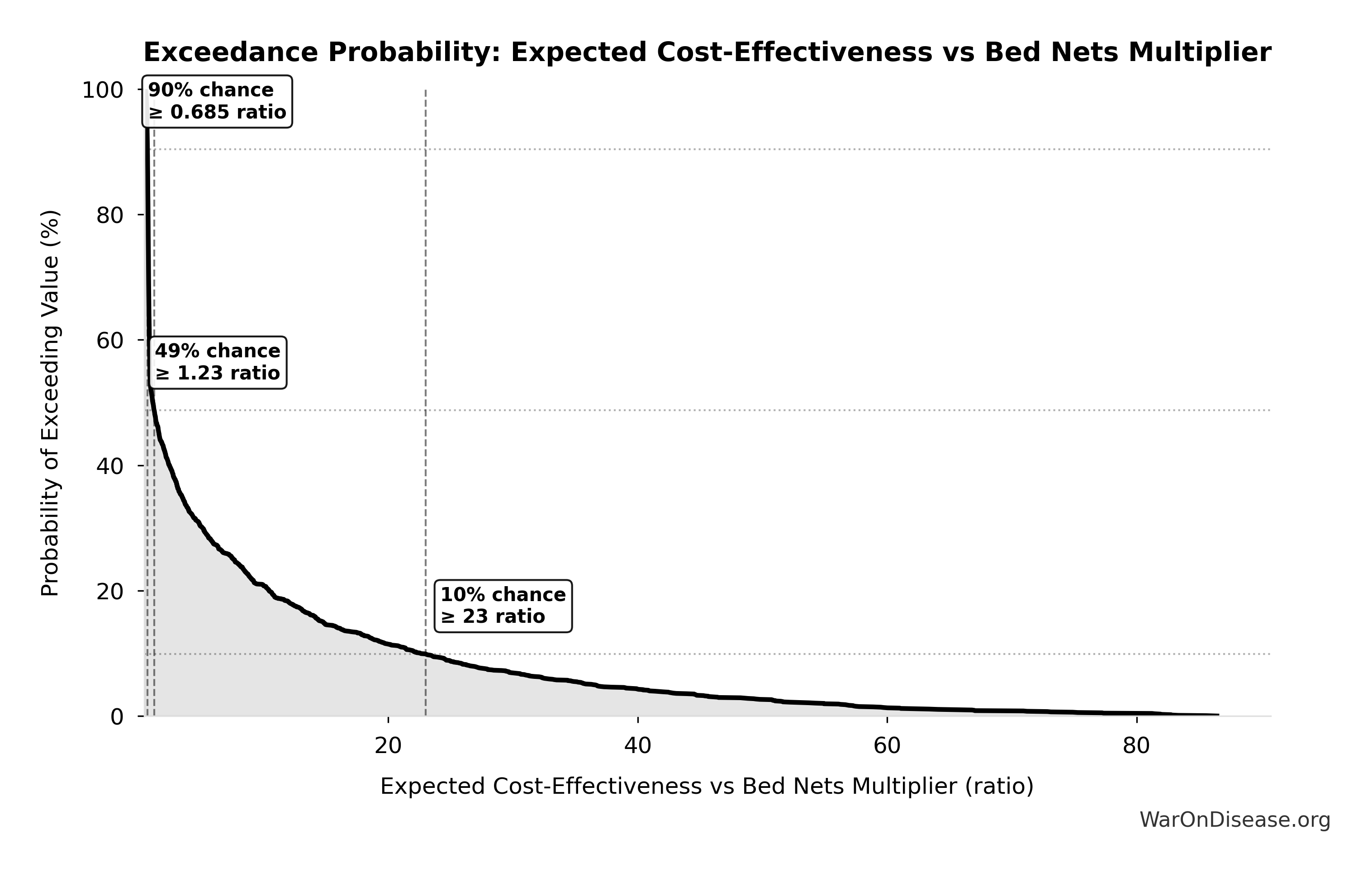
Sensitivity Indices for Treaty Trajectory vs Current Trajectory GDP Multiplier (Year 20)
Regression-based sensitivity showing which inputs explain the most variance in the output.
| Input Parameter | Sensitivity Coefficient | Interpretation |
|---|---|---|
| Treaty Trajectory GDP at Year 20 (USD) | 1.0000 | Strong driver |
| Current Trajectory GDP at Year 20 (USD) | -0.0000 | Minimal effect |
Interpretation: Standardized coefficients show the change in output (in SD units) per 1 SD change in input. Values near ±1 indicate strong influence; values exceeding ±1 may occur with correlated inputs.
Monte Carlo Distribution
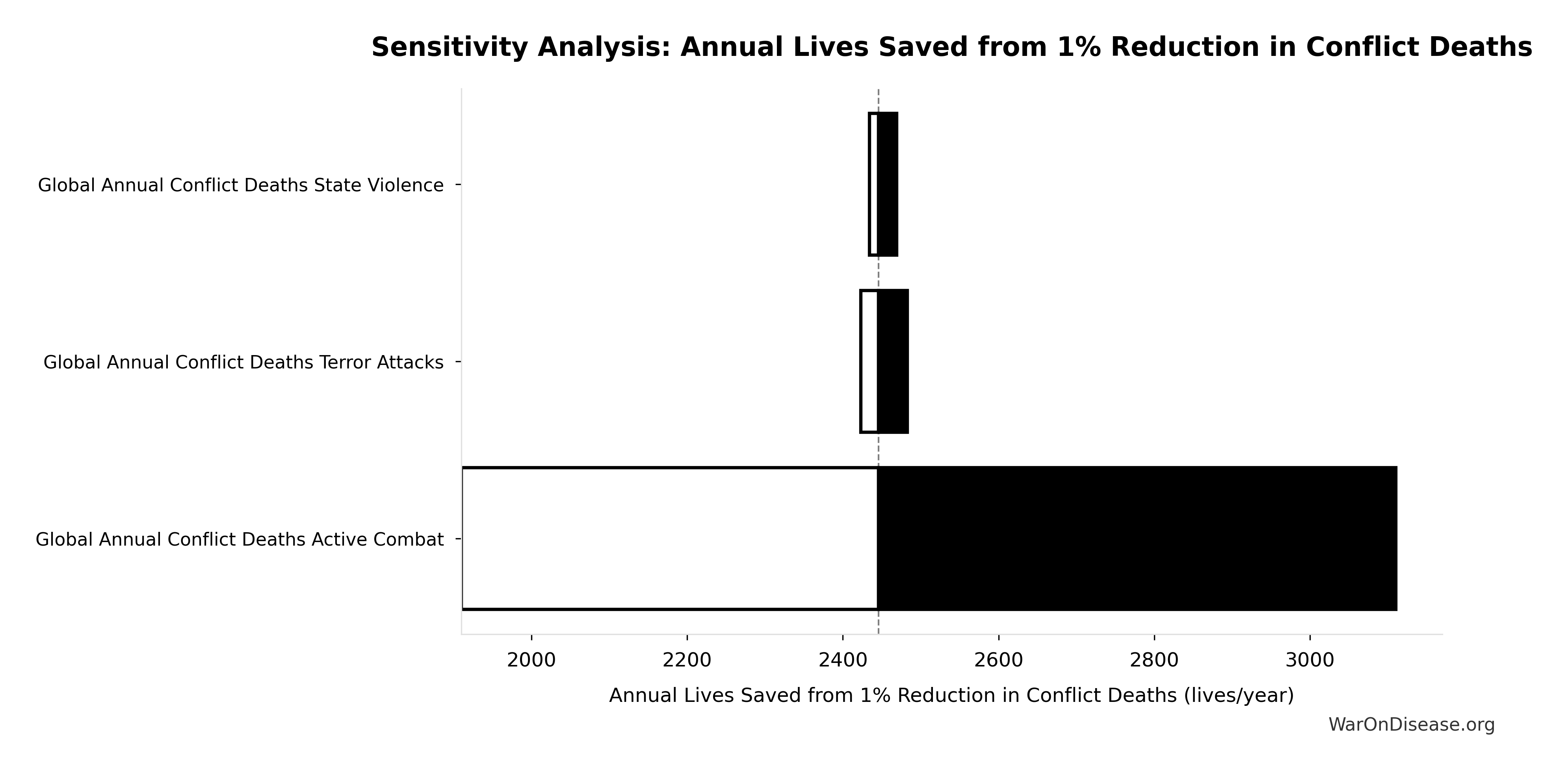
Simulation Results Summary: Treaty Trajectory vs Current Trajectory GDP Multiplier (Year 20)
| Statistic | Value |
|---|---|
| Baseline (deterministic) | 16.5x |
| Mean (expected value) | 22.6x |
| Median (50th percentile) | 16.4x |
| Standard Deviation | 18.8x |
| 90% Range (5th-95th percentile) | [5.17x, 64.9x] |
The histogram shows the distribution of Treaty Trajectory vs Current Trajectory GDP Multiplier (Year 20) across 10,000 Monte Carlo simulations. The CDF (right) shows the probability of the outcome exceeding any given value, which is useful for risk assessment.
Exceedance Probability
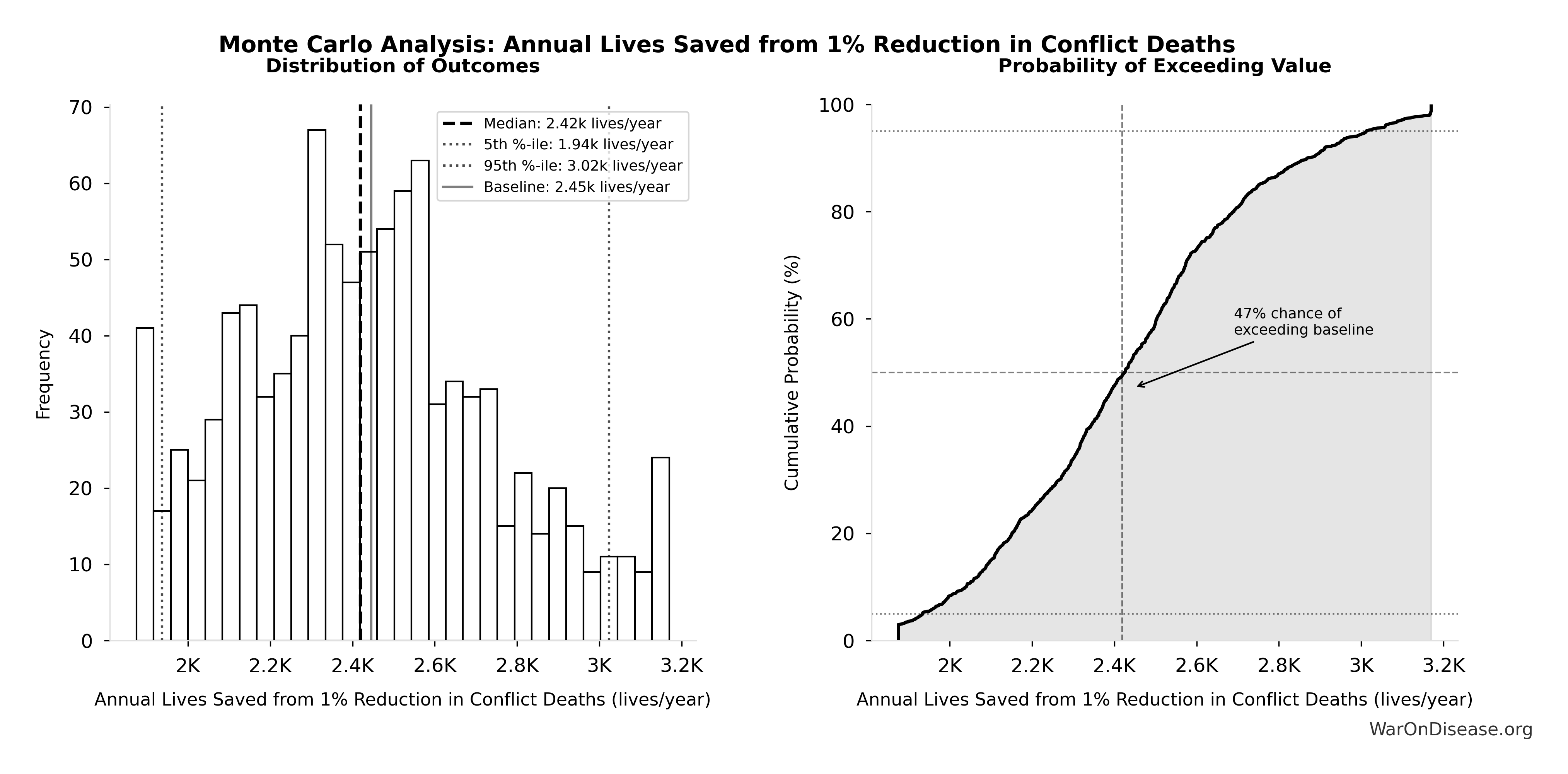
This exceedance probability chart shows the likelihood that Treaty Trajectory vs Current Trajectory GDP Multiplier (Year 20) will exceed any given threshold. Higher curves indicate more favorable outcomes with greater certainty.
Treaty Trajectory GDP at Year 20: $3.11 quadrillion
Note📊 Details
Projected global GDP at year 20 under the Treaty Trajectory: military-to-science reallocation plus disease-burden recovery only. Excludes non-health dysfunction-capital reallocation to isolate the lower-political-baggage channel.
Inputs:
- Global GDP (2025) 📊: $115T
- Baseline Global GDP Growth Rate: 2.5%
- Wishonia Military Reallocation Physical Max Share 🔢: 87.6%
- GDP Growth Boost at 30% Military Reallocation: 5.5% (95% CI: 3.5% - 7.5%)
- R&D Spillover Multiplier: 2x (95% CI: 1.5x - 2.5x)
- Wishonia Disease Cure Fraction (20yr, Full Implementation) 🔢: 100%
- Disease Burden as % of GDP 📊: 13%
\[ \begin{gathered} GDP_{treaty,20} \\ = GDP_0(1+g_{treaty,ramp})^3(1+g_{treaty,full})^{17} \end{gathered} \]
✓ High confidence
Sensitivity Analysis
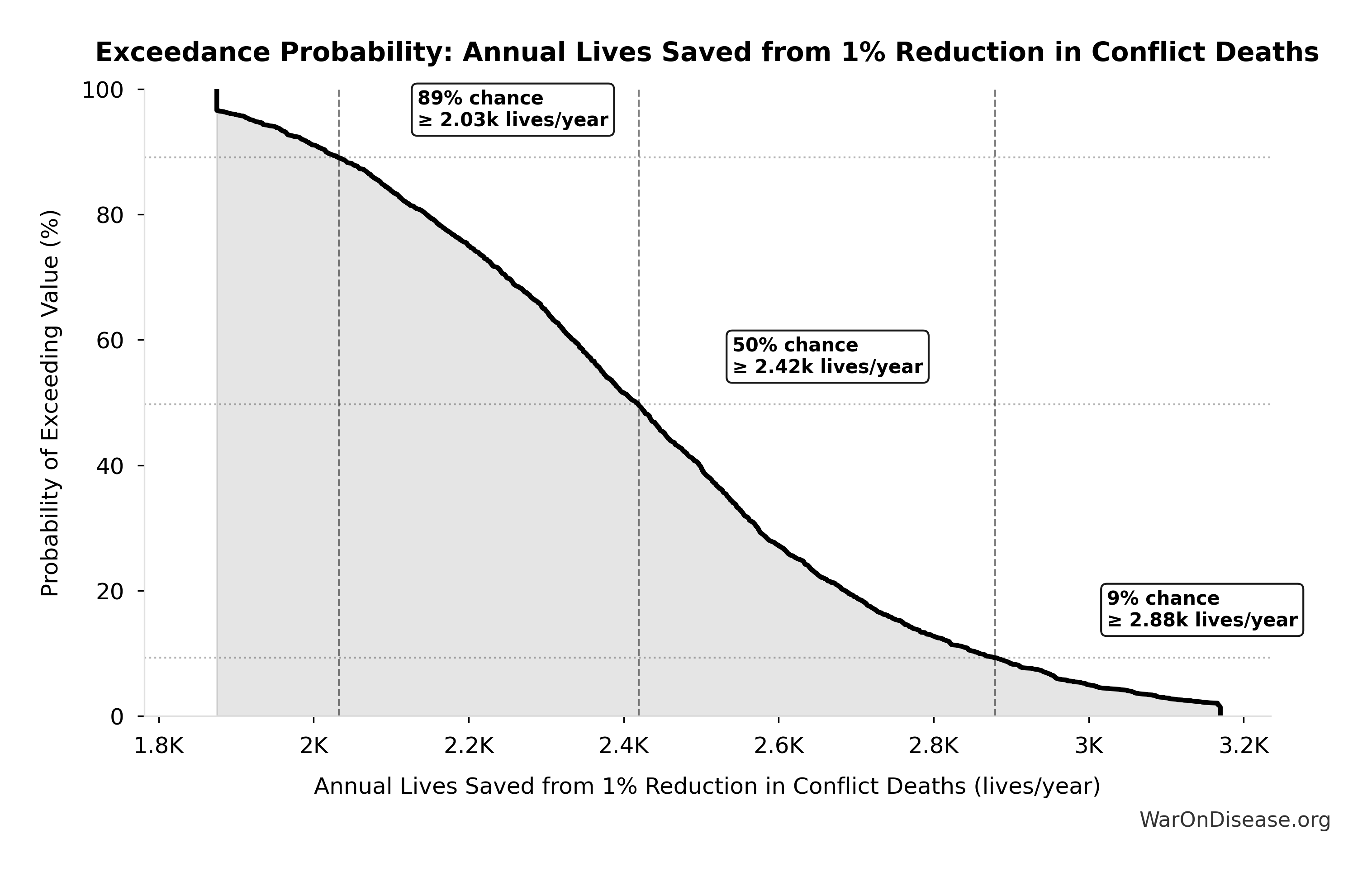
Sensitivity Indices for Treaty Trajectory GDP at Year 20
Regression-based sensitivity showing which inputs explain the most variance in the output.
| Input Parameter | Sensitivity Coefficient | Interpretation |
|---|---|---|
| GDP Growth Boost at 30% Military Reallocation (rate) | 1.8871 | Strong driver |
| R&D Spillover Multiplier (x) | -1.0000 | Strong driver |
Interpretation: Standardized coefficients show the change in output (in SD units) per 1 SD change in input. Values near ±1 indicate strong influence; values exceeding ±1 may occur with correlated inputs.
Monte Carlo Distribution
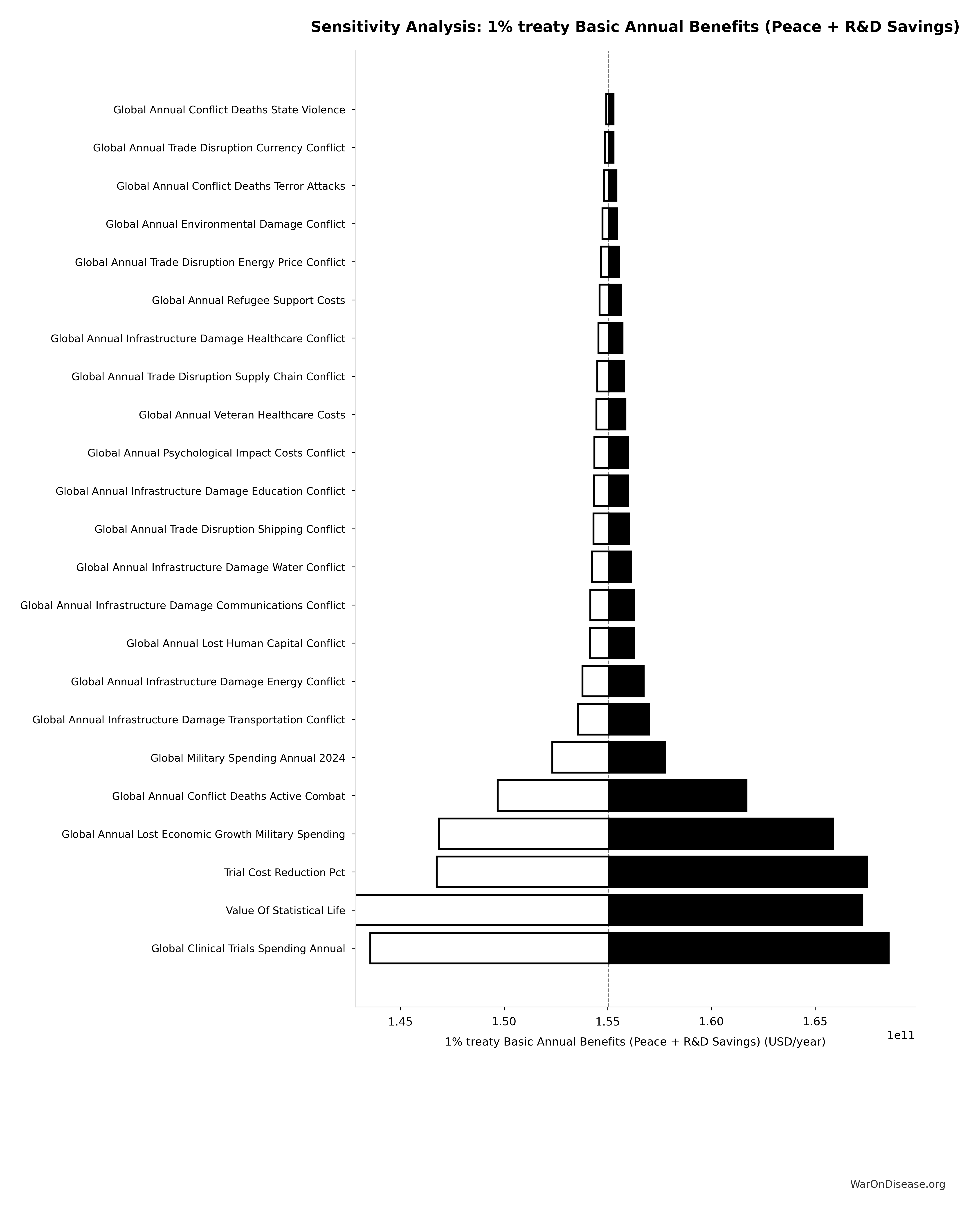
Simulation Results Summary: Treaty Trajectory GDP at Year 20
| Statistic | Value |
|---|---|
| Baseline (deterministic) | $3.11 quadrillion |
| Mean (expected value) | $4.25 quadrillion |
| Median (50th percentile) | $3.08 quadrillion |
| Standard Deviation | $3.54 quadrillion |
| 90% Range (5th-95th percentile) | [$974T, $12.2 quadrillion] |
The histogram shows the distribution of Treaty Trajectory GDP at Year 20 across 10,000 Monte Carlo simulations. The CDF (right) shows the probability of the outcome exceeding any given value, which is useful for risk assessment.
Exceedance Probability
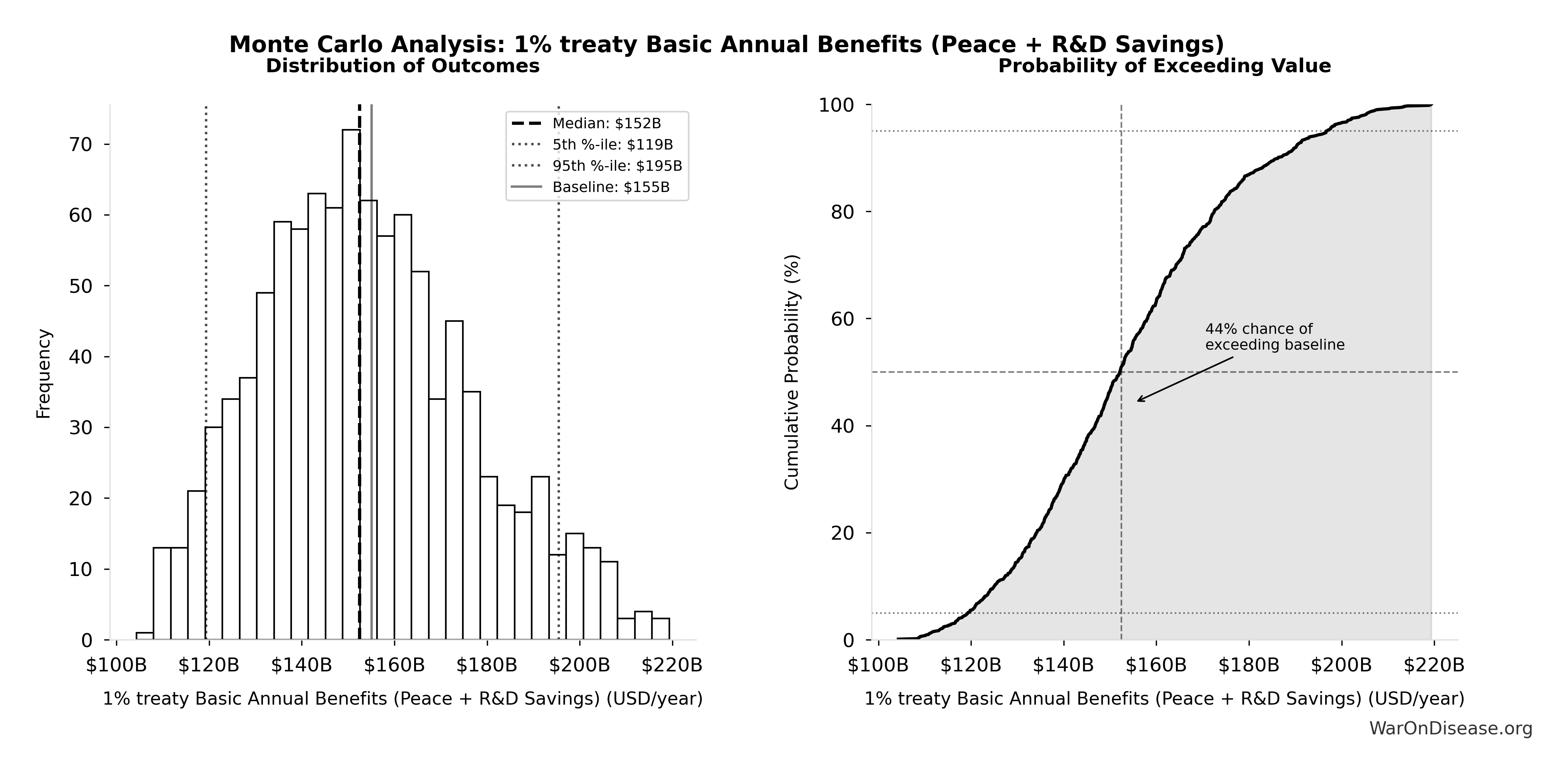
This exceedance probability chart shows the likelihood that Treaty Trajectory GDP at Year 20 will exceed any given threshold. Higher curves indicate more favorable outcomes with greater certainty.
Cost-Effectiveness vs Bed Nets Multiplier: 50.3kx
Note📊 Details
How many times more cost-effective than bed nets (using bed net cost per DALY midpoint estimate)
Inputs:
- Bed Nets Cost per DALY 📊: $89 (95% CI: $78 - $100)
- Cost per DALY Averted (Elimination of Efficacy Lag Plus Earlier Treatment Discovery from Increased Trial Throughput) 🔢: $0.00177
\[ \begin{gathered} k_{treaty:nets} \\ = \frac{Cost_{nets}}{Cost_{treaty,DALY}} \\ = \frac{\$89}{\$0.00177} \\ = 50{,}300 \end{gathered} \] where: \[ \begin{gathered} Cost_{treaty,DALY} \\ = \frac{Cost_{campaign}}{DALYs_{max}} \\ = \frac{\$1B}{565B} \\ = \$0.00177 \end{gathered} \] where: \[ \begin{gathered} Cost_{campaign} \\ = Budget_{viral,base} + Budget_{lobby,treaty} \\ + Budget_{reserve} \\ = \$250M + \$650M + \$100M \\ = \$1B \end{gathered} \] where: \[ \begin{gathered} DALYs_{max} \\ = DALYs_{global,ann} \times Pct_{avoid,DALY} \times T_{accel,max} \\ = 2.88B \times 92.6\% \times 212 \\ = 565B \end{gathered} \] where: \[ T_{accel,max} = T_{accel} + T_{lag} = 204 + 8.2 = 212 \] where: \[ \begin{gathered} T_{accel} \\ = T_{first,SQ} \times \left(1 - \frac{1}{k_{capacity}}\right) \\ = 222 \times \left(1 - \frac{1}{12.3}\right) \\ = 204 \end{gathered} \] where: \[ \begin{gathered} T_{first,SQ} \\ = T_{queue,SQ} \times 0.5 \\ = 443 \times 0.5 \\ = 222 \end{gathered} \] where: \[ \begin{gathered} T_{queue,SQ} \\ = \frac{N_{untreated}}{Treatments_{new,ann}} \\ = \frac{6{,}650}{15} \\ = 443 \end{gathered} \] where: \[ \begin{gathered} N_{untreated} \\ = N_{rare} \times 0.95 \\ = 7{,}000 \times 0.95 \\ = 6{,}650 \end{gathered} \] where: \[ \begin{gathered} k_{capacity} \\ = \frac{N_{fundable,dFDA}}{Slots_{curr}} \\ = \frac{23.4M}{1.9M} \\ = 12.3 \end{gathered} \] where: \[ \begin{gathered} N_{fundable,dFDA} \\ = \frac{Subsidies_{dFDA,ann}}{Cost_{pragmatic,pt}} \\ = \frac{\$21.8B}{\$929} \\ = 23.4M \end{gathered} \] where: \[ \begin{gathered} Subsidies_{dFDA,ann} \\ = Funding_{dFDA,ann} - OPEX_{dFDA} \\ = \$21.8B - \$40M \\ = \$21.8B \end{gathered} \] where: \[ \begin{gathered} OPEX_{dFDA} \\ = Cost_{platform} + Cost_{staff} + Cost_{infra} \\ + Cost_{regulatory} + Cost_{community} \\ = \$15M + \$10M + \$8M + \$5M + \$2M \\ = \$40M \end{gathered} \] ✓ High confidence
Sensitivity Analysis
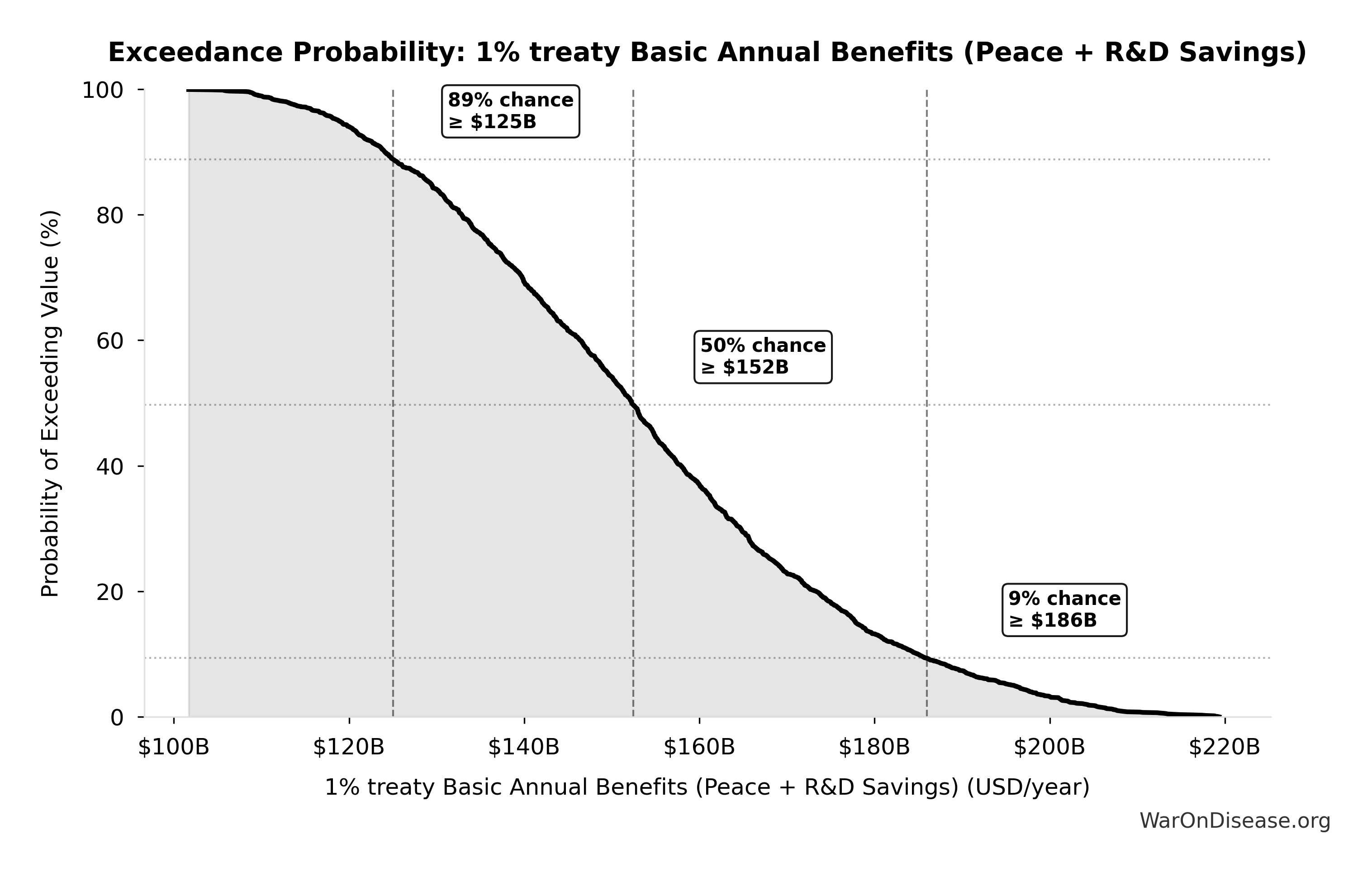
Sensitivity Indices for Cost-Effectiveness vs Bed Nets Multiplier
Regression-based sensitivity showing which inputs explain the most variance in the output.
| Input Parameter | Sensitivity Coefficient | Interpretation |
|---|---|---|
| Bed Nets Cost per DALY (USD/DALY) | -0.8683 | Strong driver |
| Cost per DALY Averted (Elimination of Efficacy Lag Plus Earlier Treatment Discovery from Increased Trial Throughput) (USD/DALY) | -0.0850 | Minimal effect |
Interpretation: Standardized coefficients show the change in output (in SD units) per 1 SD change in input. Values near ±1 indicate strong influence; values exceeding ±1 may occur with correlated inputs.
Monte Carlo Distribution
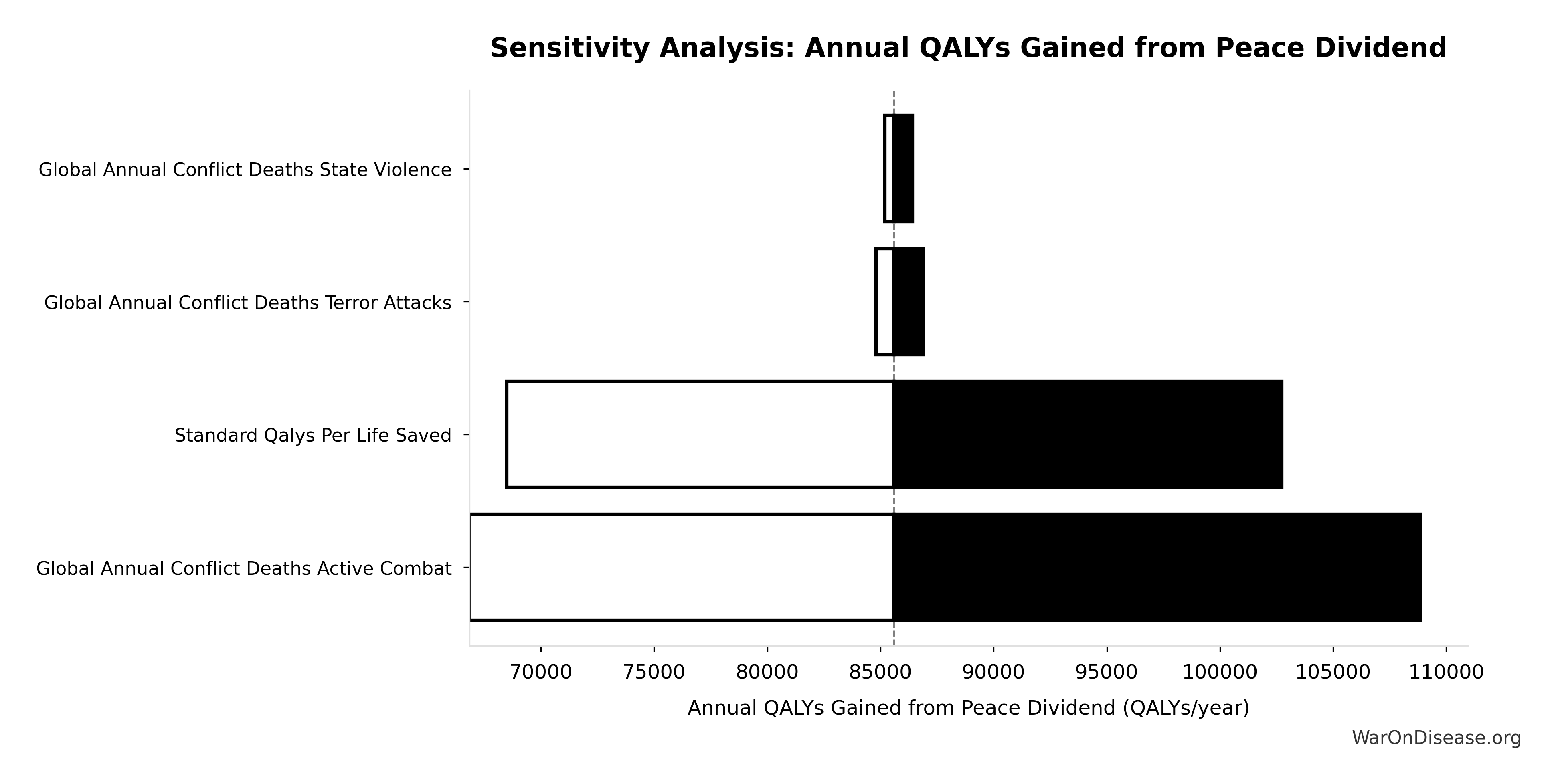
Simulation Results Summary: Cost-Effectiveness vs Bed Nets Multiplier
| Statistic | Value |
|---|---|
| Baseline (deterministic) | 50.3kx |
| Mean (expected value) | 59.9kx |
| Median (50th percentile) | 56.9kx |
| Standard Deviation | 25.0kx |
| 90% Range (5th-95th percentile) | [23.8kx, 111.7kx] |
The histogram shows the distribution of Cost-Effectiveness vs Bed Nets Multiplier across 10,000 Monte Carlo simulations. The CDF (right) shows the probability of the outcome exceeding any given value, which is useful for risk assessment.
Exceedance Probability
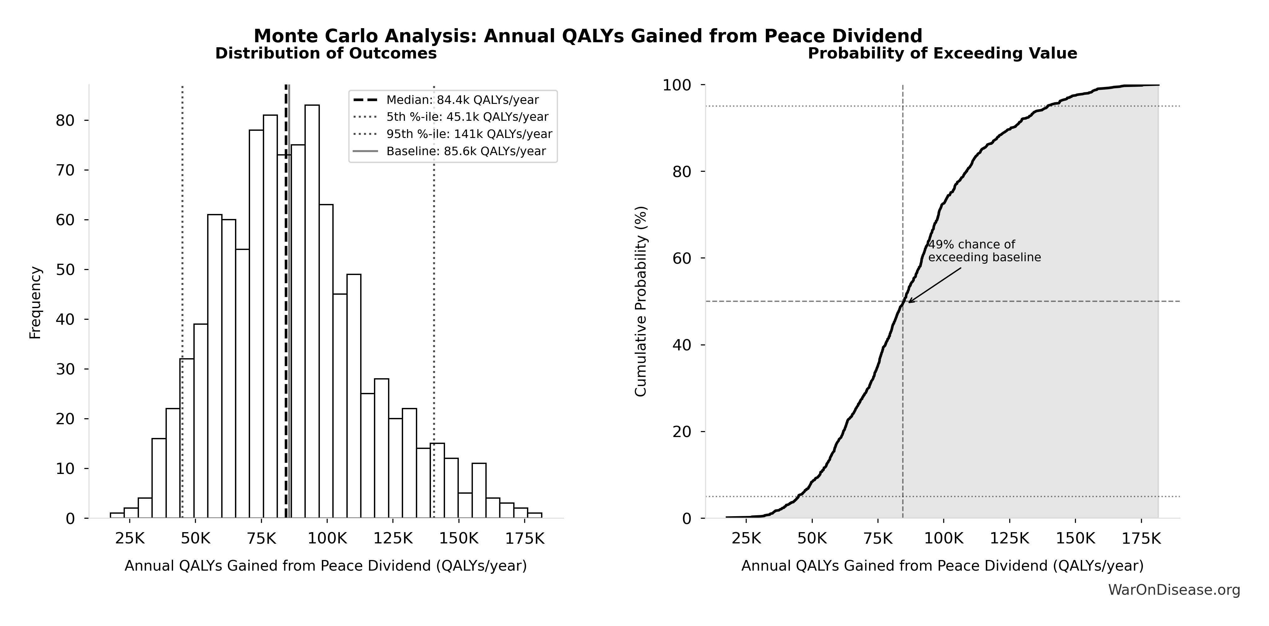
This exceedance probability chart shows the likelihood that Cost-Effectiveness vs Bed Nets Multiplier will exceed any given threshold. Higher curves indicate more favorable outcomes with greater certainty.
Treaty Campaign Leverage vs Direct Funding: 476x
Note📊 Details
How many times more cost-effective the treaty campaign is vs direct funding. Treaty campaign unlocks government funding at scale, avoiding need for philanthropists/NIH to directly commit equivalent amounts. Both approaches achieve same DALY timeline shift benefit. Treaty spreads cost across governments while building sustainable public funding infrastructure.
Inputs:
- dFDA Direct Funding Cost per DALY 🔢: $0.842
- Cost per DALY Averted (Elimination of Efficacy Lag Plus Earlier Treatment Discovery from Increased Trial Throughput) 🔢: $0.00177
\[ \begin{gathered} Leverage_{treaty} \\ = \frac{Cost_{direct,DALY}}{Cost_{treaty,DALY}} \\ = \frac{\$0.842}{\$0.00177} \\ = 476 \end{gathered} \] where: \[ \begin{gathered} Cost_{direct,DALY} \\ = \frac{NPV_{direct}}{DALYs_{max}} \\ = \frac{\$476B}{565B} \\ = \$0.842 \end{gathered} \] where: \[ NPV_{direct} = Funding_{ann} \times \frac{1 - (1+r)^{-T}}{r} \] where: \[ \begin{gathered} T_{queue,dFDA} \\ = \frac{T_{queue,SQ}}{k_{capacity}} \\ = \frac{443}{12.3} \\ = 36 \end{gathered} \] where: \[ \begin{gathered} T_{queue,SQ} \\ = \frac{N_{untreated}}{Treatments_{new,ann}} \\ = \frac{6{,}650}{15} \\ = 443 \end{gathered} \] where: \[ \begin{gathered} N_{untreated} \\ = N_{rare} \times 0.95 \\ = 7{,}000 \times 0.95 \\ = 6{,}650 \end{gathered} \] where: \[ \begin{gathered} k_{capacity} \\ = \frac{N_{fundable,dFDA}}{Slots_{curr}} \\ = \frac{23.4M}{1.9M} \\ = 12.3 \end{gathered} \] where: \[ \begin{gathered} N_{fundable,dFDA} \\ = \frac{Subsidies_{dFDA,ann}}{Cost_{pragmatic,pt}} \\ = \frac{\$21.8B}{\$929} \\ = 23.4M \end{gathered} \] where: \[ \begin{gathered} Subsidies_{dFDA,ann} \\ = Funding_{dFDA,ann} - OPEX_{dFDA} \\ = \$21.8B - \$40M \\ = \$21.8B \end{gathered} \] where: \[ \begin{gathered} OPEX_{dFDA} \\ = Cost_{platform} + Cost_{staff} + Cost_{infra} \\ + Cost_{regulatory} + Cost_{community} \\ = \$15M + \$10M + \$8M + \$5M + \$2M \\ = \$40M \end{gathered} \] where: \[ \begin{gathered} DALYs_{max} \\ = DALYs_{global,ann} \times Pct_{avoid,DALY} \times T_{accel,max} \\ = 2.88B \times 92.6\% \times 212 \\ = 565B \end{gathered} \] where: \[ T_{accel,max} = T_{accel} + T_{lag} = 204 + 8.2 = 212 \] where: \[ \begin{gathered} T_{accel} \\ = T_{first,SQ} \times \left(1 - \frac{1}{k_{capacity}}\right) \\ = 222 \times \left(1 - \frac{1}{12.3}\right) \\ = 204 \end{gathered} \] where: \[ \begin{gathered} T_{first,SQ} \\ = T_{queue,SQ} \times 0.5 \\ = 443 \times 0.5 \\ = 222 \end{gathered} \] where: \[ \begin{gathered} Cost_{treaty,DALY} \\ = \frac{Cost_{campaign}}{DALYs_{max}} \\ = \frac{\$1B}{565B} \\ = \$0.00177 \end{gathered} \] where: \[ \begin{gathered} Cost_{campaign} \\ = Budget_{viral,base} + Budget_{lobby,treaty} \\ + Budget_{reserve} \\ = \$250M + \$650M + \$100M \\ = \$1B \end{gathered} \] ✓ High confidence
Sensitivity Analysis
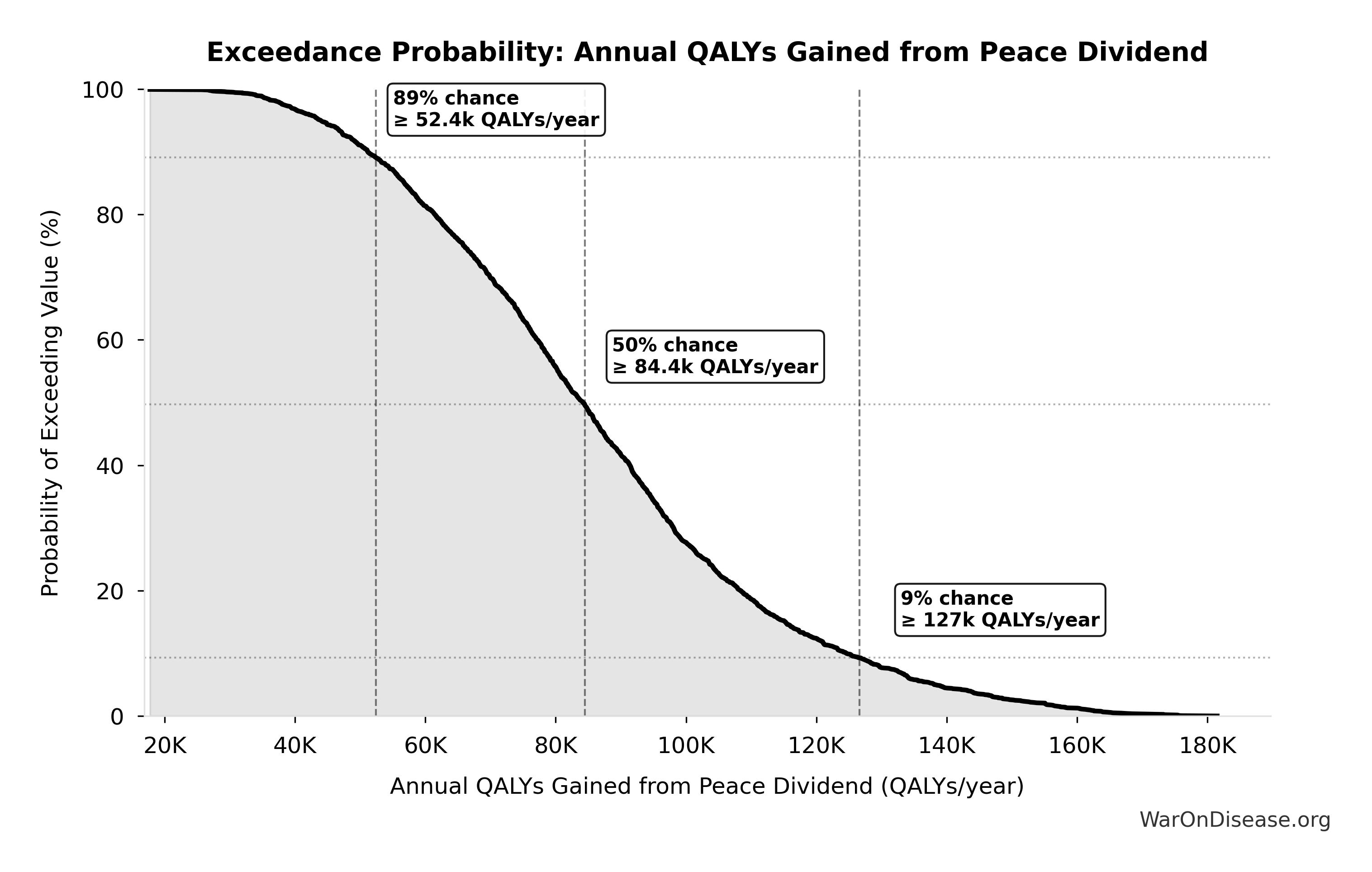
Sensitivity Indices for Treaty Campaign Leverage vs Direct Funding
Regression-based sensitivity showing which inputs explain the most variance in the output.
| Input Parameter | Sensitivity Coefficient | Interpretation |
|---|---|---|
| dFDA Direct Funding Cost per DALY (USD/DALY) | 4.1729 | Strong driver |
| Cost per DALY Averted (Elimination of Efficacy Lag Plus Earlier Treatment Discovery from Increased Trial Throughput) (USD/DALY) | -3.7762 | Strong driver |
Interpretation: Standardized coefficients show the change in output (in SD units) per 1 SD change in input. Values near ±1 indicate strong influence; values exceeding ±1 may occur with correlated inputs.
Monte Carlo Distribution
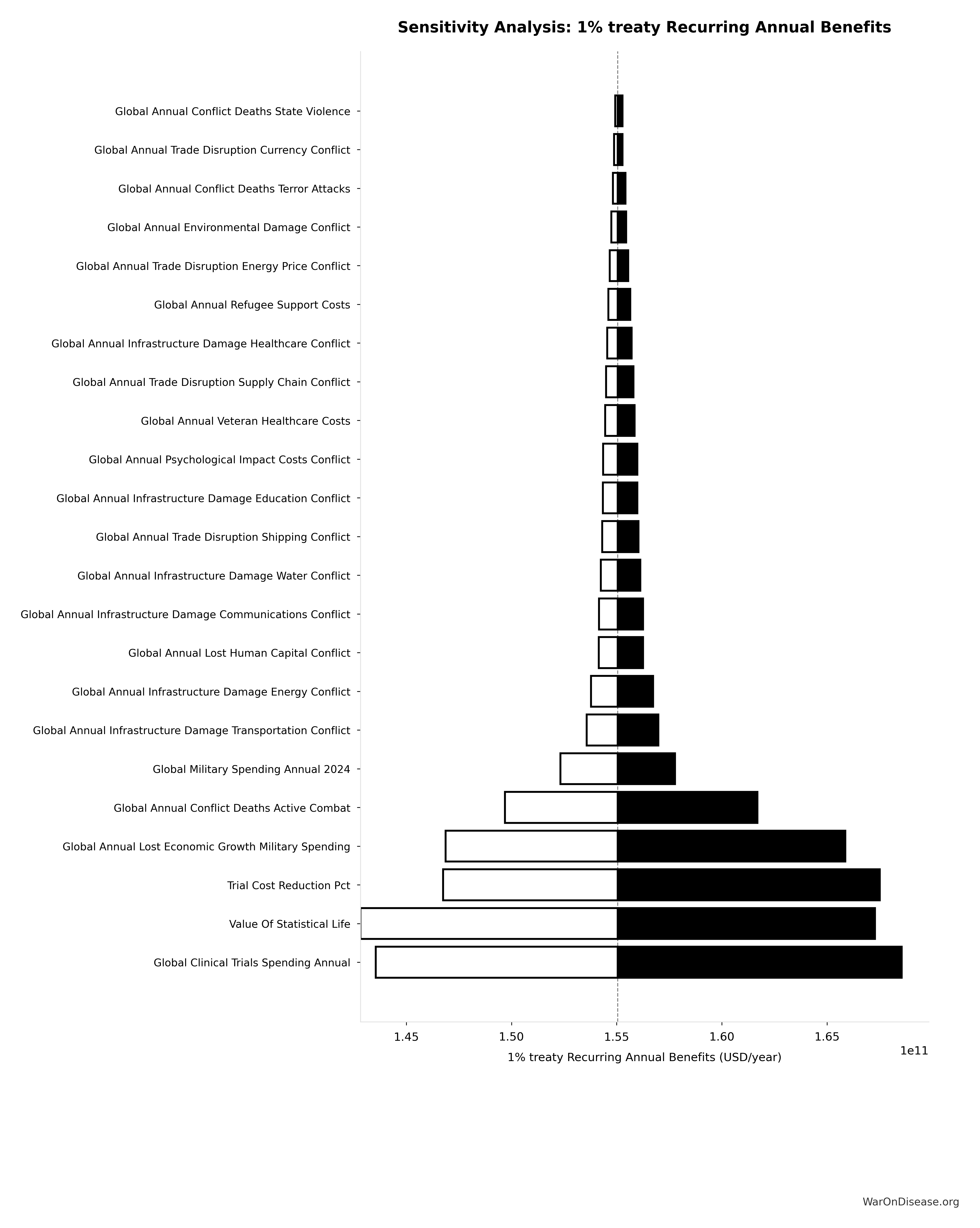
Simulation Results Summary: Treaty Campaign Leverage vs Direct Funding
| Statistic | Value |
|---|---|
| Baseline (deterministic) | 476x |
| Mean (expected value) | 421x |
| Median (50th percentile) | 438x |
| Standard Deviation | 47.5x |
| 90% Range (5th-95th percentile) | [329x, 462x] |
The histogram shows the distribution of Treaty Campaign Leverage vs Direct Funding across 10,000 Monte Carlo simulations. The CDF (right) shows the probability of the outcome exceeding any given value, which is useful for risk assessment.
Exceedance Probability

This exceedance probability chart shows the likelihood that Treaty Campaign Leverage vs Direct Funding will exceed any given threshold. Higher curves indicate more favorable outcomes with greater certainty.
Cumulative Trial Capacity Years Over 20 Years: 247 years
Note📊 Details
Cumulative trial-capacity-equivalent years over 20-year period
Inputs:
- Trial Capacity Multiplier 🔢: 12.3x
\[ \begin{gathered} Capacity_{20yr} \\ = k_{capacity} \times 20 \\ = 12.3 \times 20 \\ = 247 \end{gathered} \] where: \[ \begin{gathered} k_{capacity} \\ = \frac{N_{fundable,dFDA}}{Slots_{curr}} \\ = \frac{23.4M}{1.9M} \\ = 12.3 \end{gathered} \] where: \[ \begin{gathered} N_{fundable,dFDA} \\ = \frac{Subsidies_{dFDA,ann}}{Cost_{pragmatic,pt}} \\ = \frac{\$21.8B}{\$929} \\ = 23.4M \end{gathered} \] where: \[ \begin{gathered} Subsidies_{dFDA,ann} \\ = Funding_{dFDA,ann} - OPEX_{dFDA} \\ = \$21.8B - \$40M \\ = \$21.8B \end{gathered} \] where: \[ \begin{gathered} OPEX_{dFDA} \\ = Cost_{platform} + Cost_{staff} + Cost_{infra} \\ + Cost_{regulatory} + Cost_{community} \\ = \$15M + \$10M + \$8M + \$5M + \$2M \\ = \$40M \end{gathered} \] ✓ High confidence
Sensitivity Analysis

Sensitivity Indices for Cumulative Trial Capacity Years Over 20 Years
Regression-based sensitivity showing which inputs explain the most variance in the output.
| Input Parameter | Sensitivity Coefficient | Interpretation |
|---|---|---|
| Trial Capacity Multiplier (x) | 1.0000 | Strong driver |
Interpretation: Standardized coefficients show the change in output (in SD units) per 1 SD change in input. Values near ±1 indicate strong influence; values exceeding ±1 may occur with correlated inputs.
Monte Carlo Distribution
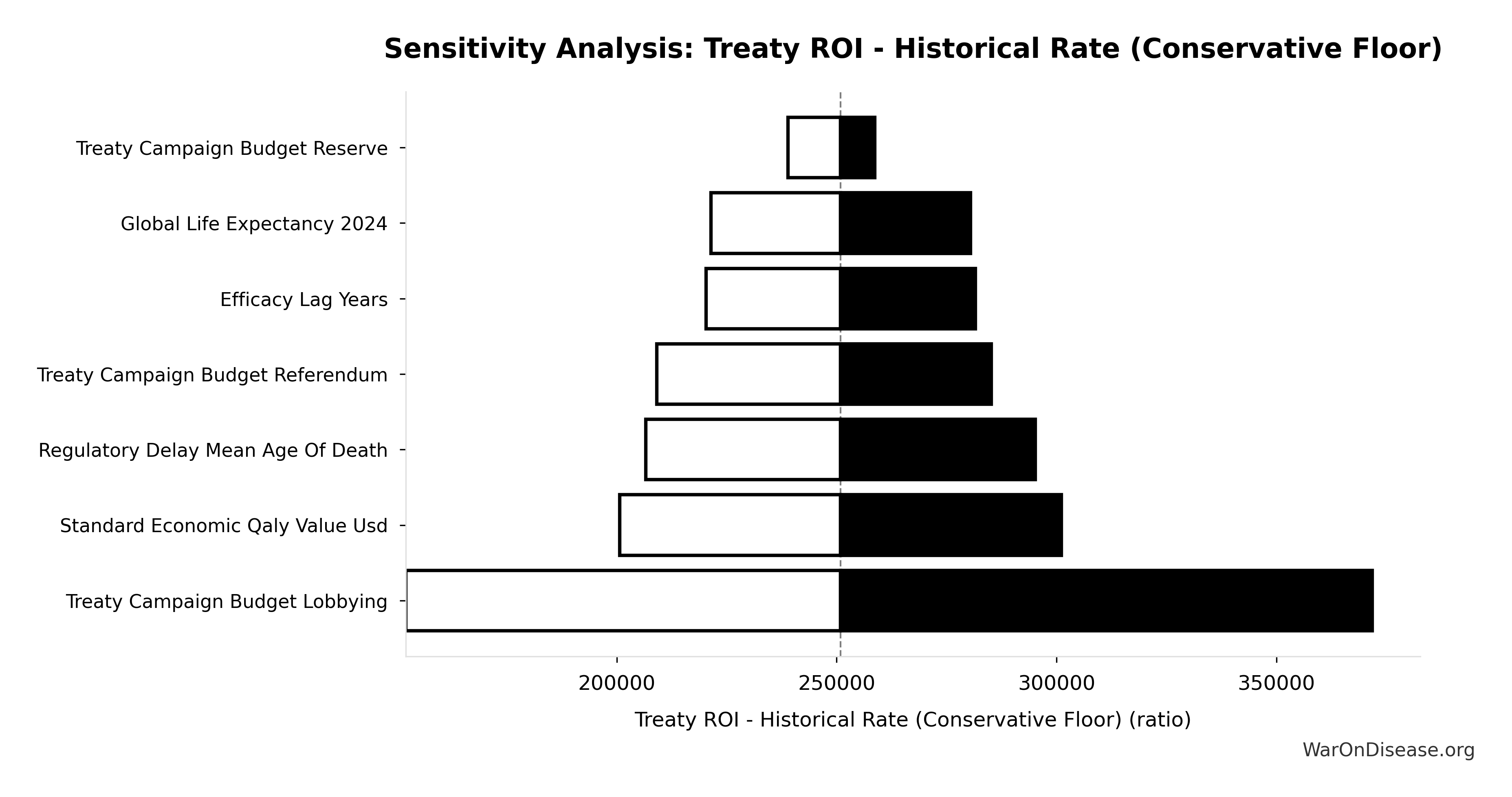
Simulation Results Summary: Cumulative Trial Capacity Years Over 20 Years
| Statistic | Value |
|---|---|
| Baseline (deterministic) | 247 |
| Mean (expected value) | 442 |
| Median (50th percentile) | 321 |
| Standard Deviation | 405 |
| 90% Range (5th-95th percentile) | [84, 1.23 thousand] |
The histogram shows the distribution of Cumulative Trial Capacity Years Over 20 Years across 10,000 Monte Carlo simulations. The CDF (right) shows the probability of the outcome exceeding any given value, which is useful for risk assessment.
Exceedance Probability
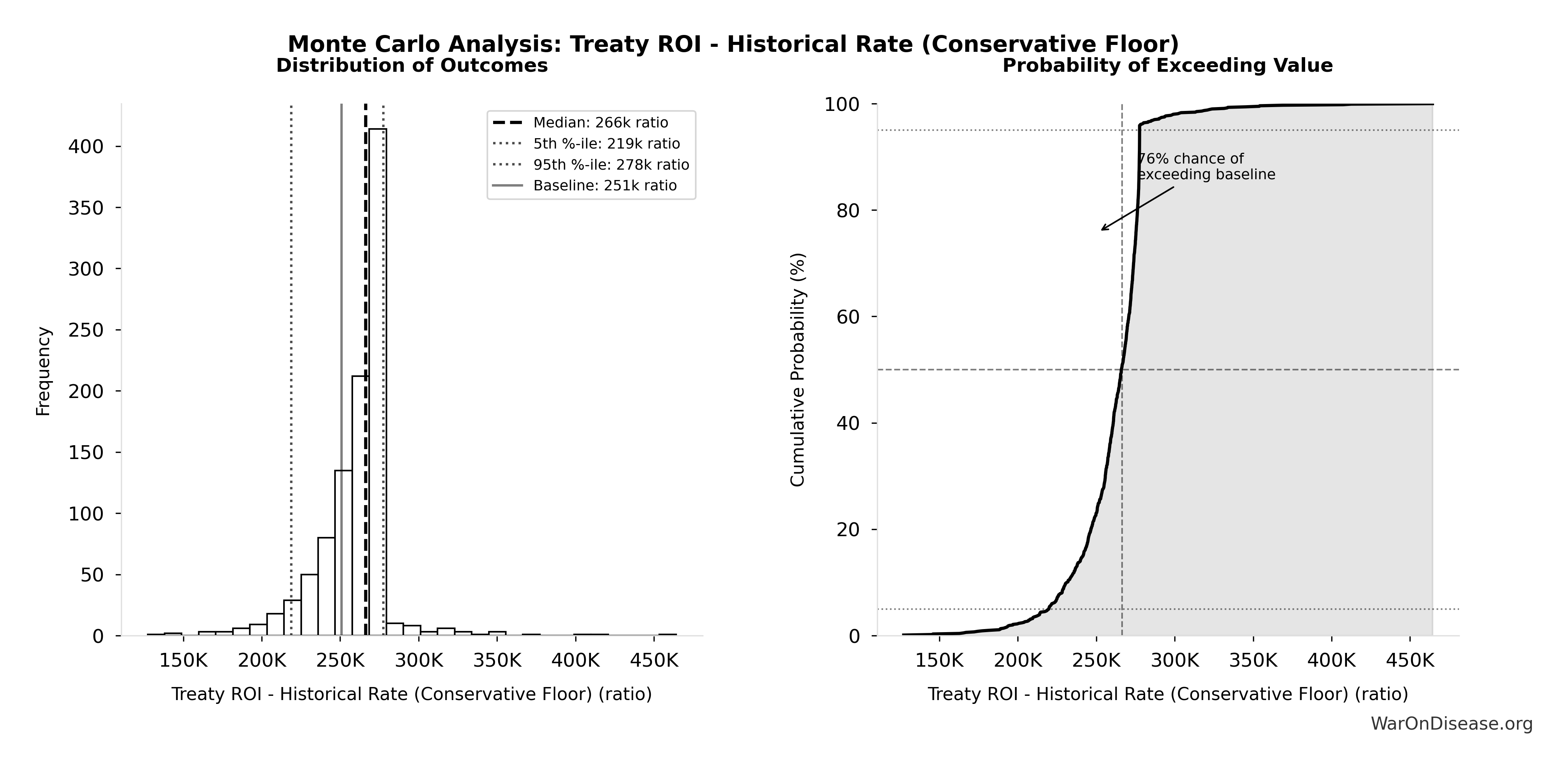
This exceedance probability chart shows the likelihood that Cumulative Trial Capacity Years Over 20 Years will exceed any given threshold. Higher curves indicate more favorable outcomes with greater certainty.
Ratio of Type II Error Cost to Type I Error Benefit: 3.07k:1
Note📊 Details
Ratio of Type II error cost to Type I error benefit (harm from delay vs. harm prevented)
Inputs:
- Total DALYs Lost from Disease Eradication Delay 🔢: 7.94 billion DALYs
- Maximum DALYs Saved by FDA Preventing Unsafe Drugs (1962-2024) 🔢: 2.59 million DALYs
\[ \begin{gathered} Ratio_{TypeII} \\ = \frac{DALYs_{lag}}{DALY_{TypeI}} \\ = \frac{7.94B}{2.59M} \\ = 3{,}070 \end{gathered} \] where: \[ DALYs_{lag} = YLL_{lag} + YLD_{lag} = 7.07B + 873M = 7.94B \] where: \[ \begin{gathered} YLL_{lag} \\ = Deaths_{lag} \times (LE_{global} - Age_{death,delay}) \\ = 416M \times (79 - 62) \\ = 7.07B \end{gathered} \] where: \[ \begin{gathered} Deaths_{lag} \\ = T_{lag} \times Deaths_{disease,daily} \times 338 \\ = 8.2 \times 150{,}000 \times 338 \\ = 416M \end{gathered} \] where: \[ \begin{gathered} YLD_{lag} \\ = Deaths_{lag} \times T_{suffering} \times DW_{chronic} \\ = 416M \times 6 \times 0.35 \\ = 873M \end{gathered} \] where: \[ \begin{gathered} DALY_{TypeI} \\ = DALY_{thal} \times 62 \\ = 41{,}800 \times 62 \\ = 2.59M \end{gathered} \] where: \[ \begin{gathered} DALY_{thal} \\ = YLD_{thal} + YLL_{thal} \\ = 13{,}000 + 28{,}800 \\ = 41{,}800 \end{gathered} \] where: \[ \begin{gathered} YLD_{thal} \\ = DW_{thal} \times N_{thal,survive} \times LE_{thal} \\ = 0.4 \times 540 \times 60 \\ = 13{,}000 \end{gathered} \] where: \[ \begin{gathered} N_{thal,survive} \\ = N_{thal,US,prevent} \times (1 - Rate_{thal,mort}) \\ = 900 \times (1 - 40\%) \\ = 540 \end{gathered} \] where: \[ \begin{gathered} N_{thal,US,prevent} \\ = N_{thal,global} \times Pct_{US,1960} \\ = 15{,}000 \times 6\% \\ = 900 \end{gathered} \] where: \[ \begin{gathered} YLL_{thal} \\ = Deaths_{thal} \times 80 \\ = 360 \times 80 \\ = 28{,}800 \end{gathered} \] where: \[ \begin{gathered} Deaths_{thal} \\ = Rate_{thal,mort} \times N_{thal,US,prevent} \\ = 40\% \times 900 \\ = 360 \end{gathered} \] ~ Medium confidence
Sensitivity Analysis
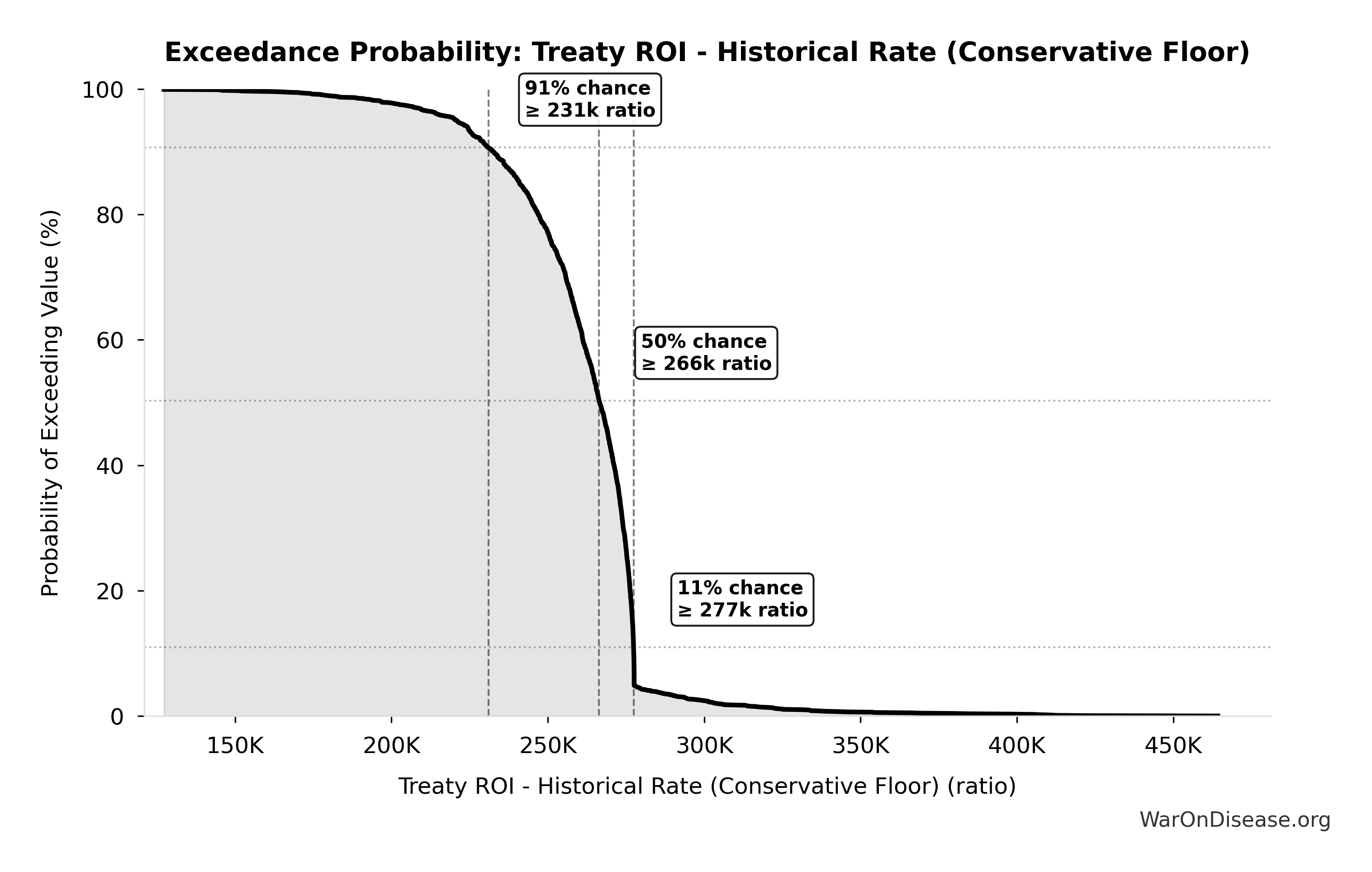
Sensitivity Indices for Ratio of Type II Error Cost to Type I Error Benefit
Regression-based sensitivity showing which inputs explain the most variance in the output.
| Input Parameter | Sensitivity Coefficient | Interpretation |
|---|---|---|
| Total DALYs Lost from Disease Eradication Delay (DALYs) | 7.2872 | Strong driver |
| Maximum DALYs Saved by FDA Preventing Unsafe Drugs (1962-2024) (DALYs) | -7.1207 | Strong driver |
Interpretation: Standardized coefficients show the change in output (in SD units) per 1 SD change in input. Values near ±1 indicate strong influence; values exceeding ±1 may occur with correlated inputs.
Monte Carlo Distribution
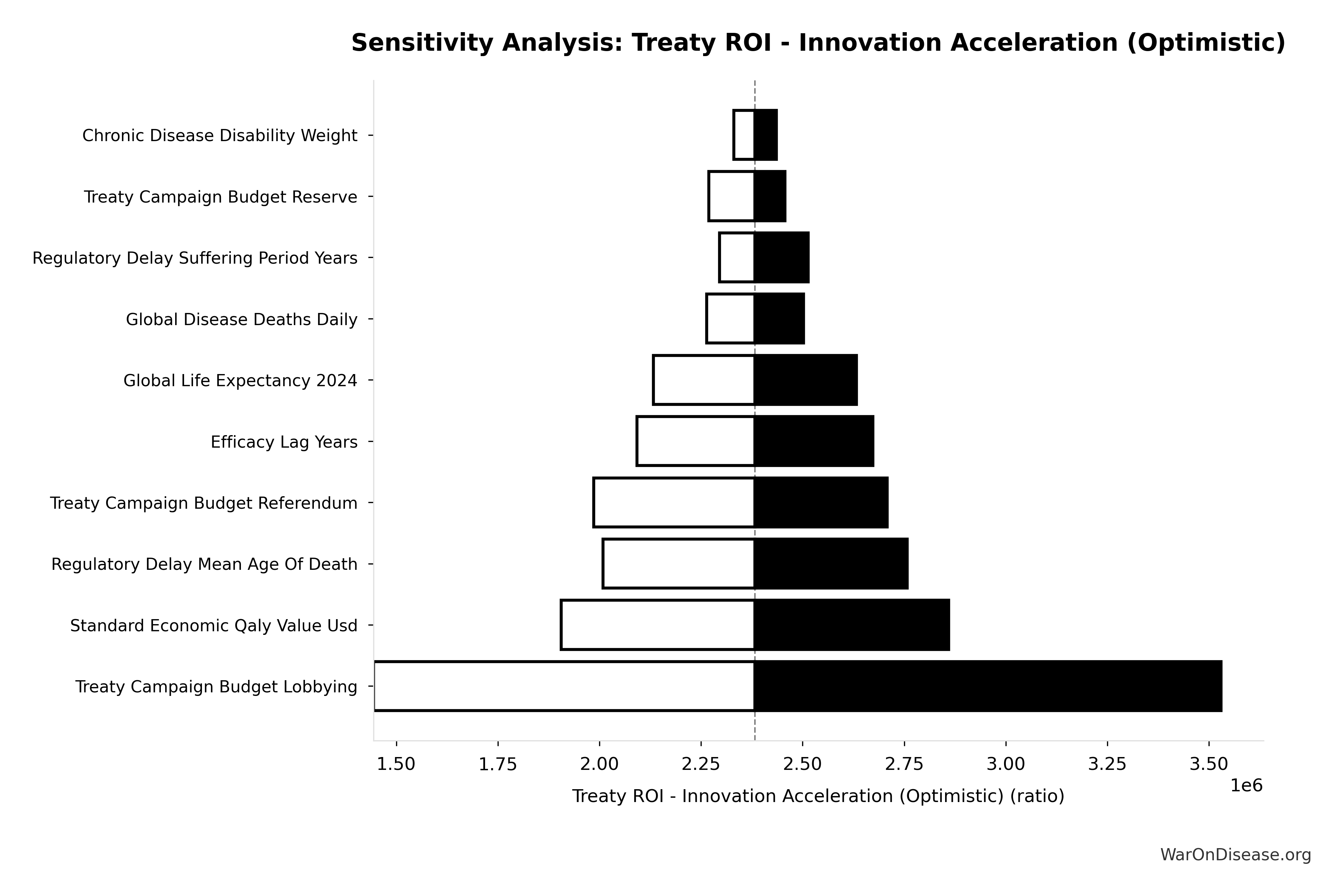
Simulation Results Summary: Ratio of Type II Error Cost to Type I Error Benefit
| Statistic | Value |
|---|---|
| Baseline (deterministic) | 3.07k:1 |
| Mean (expected value) | 3.05k:1 |
| Median (50th percentile) | 3.09k:1 |
| Standard Deviation | 101:1 |
| 90% Range (5th-95th percentile) | [2.88k:1, 3.12k:1] |
The histogram shows the distribution of Ratio of Type II Error Cost to Type I Error Benefit across 10,000 Monte Carlo simulations. The CDF (right) shows the probability of the outcome exceeding any given value, which is useful for risk assessment.
Exceedance Probability
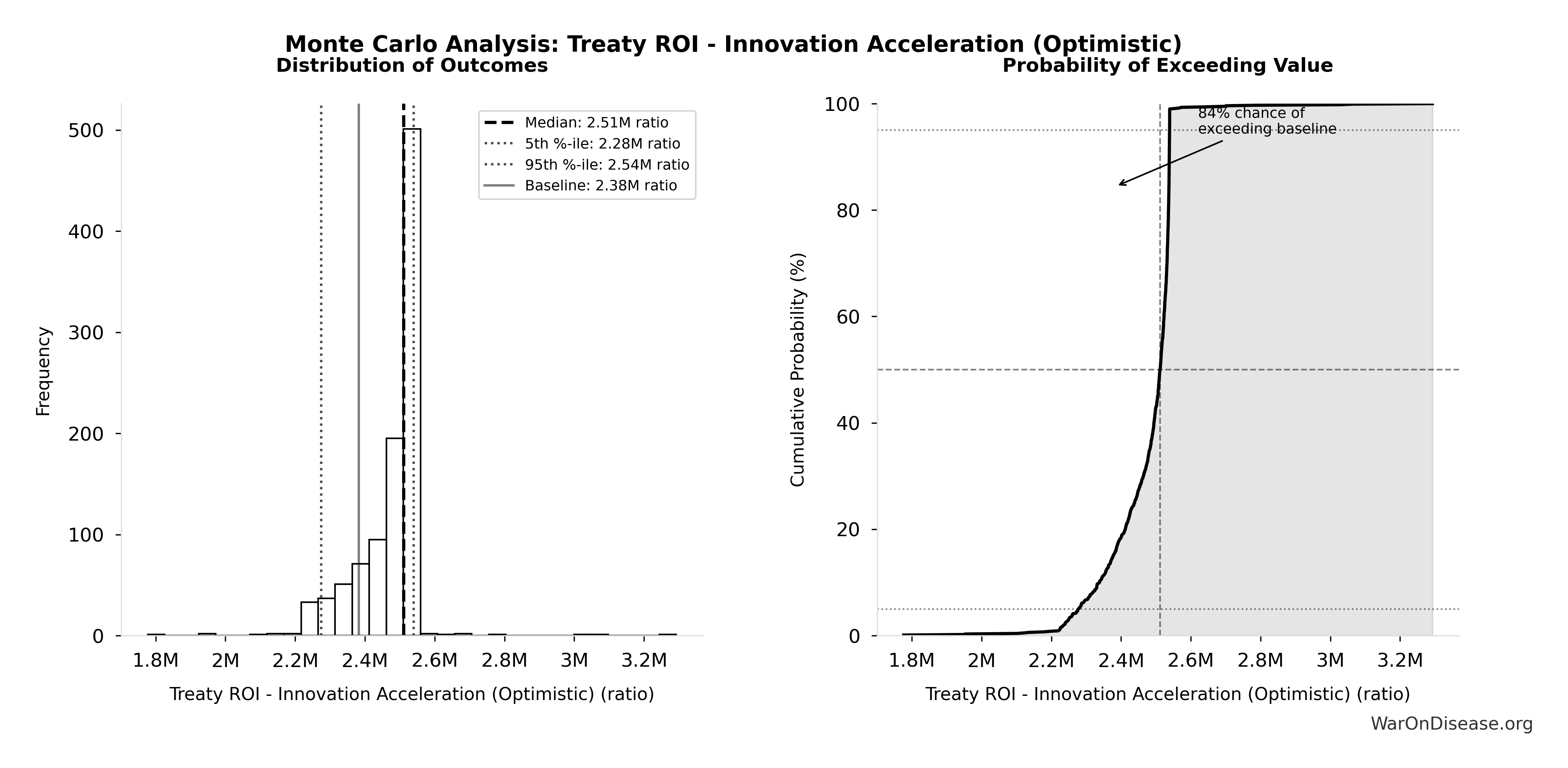
This exceedance probability chart shows the likelihood that Ratio of Type II Error Cost to Type I Error Benefit will exceed any given threshold. Higher curves indicate more favorable outcomes with greater certainty.
Maximum DALYs Saved by FDA Preventing Unsafe Drugs (1962-2024): 2.59 million DALYs
Note📊 Details
Maximum DALYs saved by FDA preventing unsafe drugs over 62-year period 1962-2024 (extreme overestimate: one Thalidomide-scale event per year)
Inputs:
- Thalidomide DALYs Per Event 🔢: 41.8 thousand DALYs
\[ \begin{gathered} DALY_{TypeI} \\ = DALY_{thal} \times 62 \\ = 41{,}800 \times 62 \\ = 2.59M \end{gathered} \] where: \[ \begin{gathered} DALY_{thal} \\ = YLD_{thal} + YLL_{thal} \\ = 13{,}000 + 28{,}800 \\ = 41{,}800 \end{gathered} \] where: \[ \begin{gathered} YLD_{thal} \\ = DW_{thal} \times N_{thal,survive} \times LE_{thal} \\ = 0.4 \times 540 \times 60 \\ = 13{,}000 \end{gathered} \] where: \[ \begin{gathered} N_{thal,survive} \\ = N_{thal,US,prevent} \times (1 - Rate_{thal,mort}) \\ = 900 \times (1 - 40\%) \\ = 540 \end{gathered} \] where: \[ \begin{gathered} N_{thal,US,prevent} \\ = N_{thal,global} \times Pct_{US,1960} \\ = 15{,}000 \times 6\% \\ = 900 \end{gathered} \] where: \[ \begin{gathered} YLL_{thal} \\ = Deaths_{thal} \times 80 \\ = 360 \times 80 \\ = 28{,}800 \end{gathered} \] where: \[ \begin{gathered} Deaths_{thal} \\ = Rate_{thal,mort} \times N_{thal,US,prevent} \\ = 40\% \times 900 \\ = 360 \end{gathered} \] ? Low confidence
Sensitivity Analysis
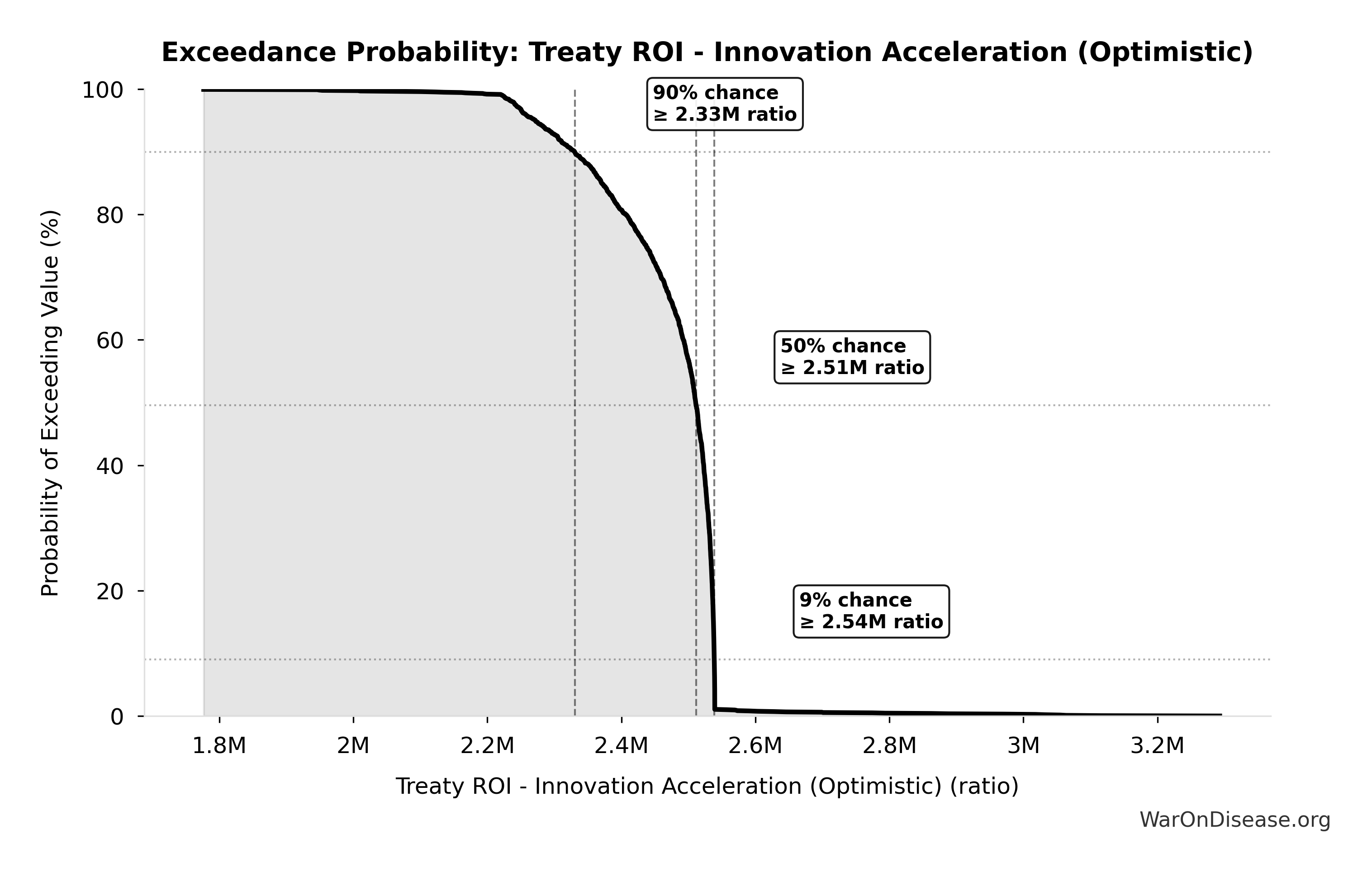
Sensitivity Indices for Maximum DALYs Saved by FDA Preventing Unsafe Drugs (1962-2024)
Regression-based sensitivity showing which inputs explain the most variance in the output.
| Input Parameter | Sensitivity Coefficient | Interpretation |
|---|---|---|
| Thalidomide DALYs Per Event (DALYs) | 1.0000 | Strong driver |
Interpretation: Standardized coefficients show the change in output (in SD units) per 1 SD change in input. Values near ±1 indicate strong influence; values exceeding ±1 may occur with correlated inputs.
Monte Carlo Distribution

Simulation Results Summary: Maximum DALYs Saved by FDA Preventing Unsafe Drugs (1962-2024)
| Statistic | Value |
|---|---|
| Baseline (deterministic) | 2.59 million |
| Mean (expected value) | 2.63 million |
| Median (50th percentile) | 2.53 million |
| Standard Deviation | 754 thousand |
| 90% Range (5th-95th percentile) | [1.54 million, 4.16 million] |
The histogram shows the distribution of Maximum DALYs Saved by FDA Preventing Unsafe Drugs (1962-2024) across 10,000 Monte Carlo simulations. The CDF (right) shows the probability of the outcome exceeding any given value, which is useful for risk assessment.
Exceedance Probability

This exceedance probability chart shows the likelihood that Maximum DALYs Saved by FDA Preventing Unsafe Drugs (1962-2024) will exceed any given threshold. Higher curves indicate more favorable outcomes with greater certainty.
Unexplored Therapeutic Frontier: 99.7%
Note📊 Details
Fraction of possible drug-disease space that remains unexplored (>99%)
Inputs:
- Tested Drug-Disease Relationships: 32.5 thousand relationships (95% CI: 15 thousand relationships - 50 thousand relationships)
- Possible Drug-Disease Combinations 🔢: 9.5 million combinations
\[ \begin{gathered} Ratio_{unexplored} \\ = 1 - \frac{N_{tested}}{N_{combos}} \\ = 1 - \frac{32{,}500}{9.5M} \\ = 99.7\% \end{gathered} \] where: \[ \begin{gathered} N_{combos} \\ = N_{safe} \times N_{diseases,trial} \\ = 9{,}500 \times 1{,}000 \\ = 9.5M \end{gathered} \] ✓ High confidence
Sensitivity Analysis

Sensitivity Indices for Unexplored Therapeutic Frontier
Regression-based sensitivity showing which inputs explain the most variance in the output.
| Input Parameter | Sensitivity Coefficient | Interpretation |
|---|---|---|
| Tested Drug-Disease Relationships (relationships) | -1.0000 | Strong driver |
Interpretation: Standardized coefficients show the change in output (in SD units) per 1 SD change in input. Values near ±1 indicate strong influence; values exceeding ±1 may occur with correlated inputs.
Monte Carlo Distribution
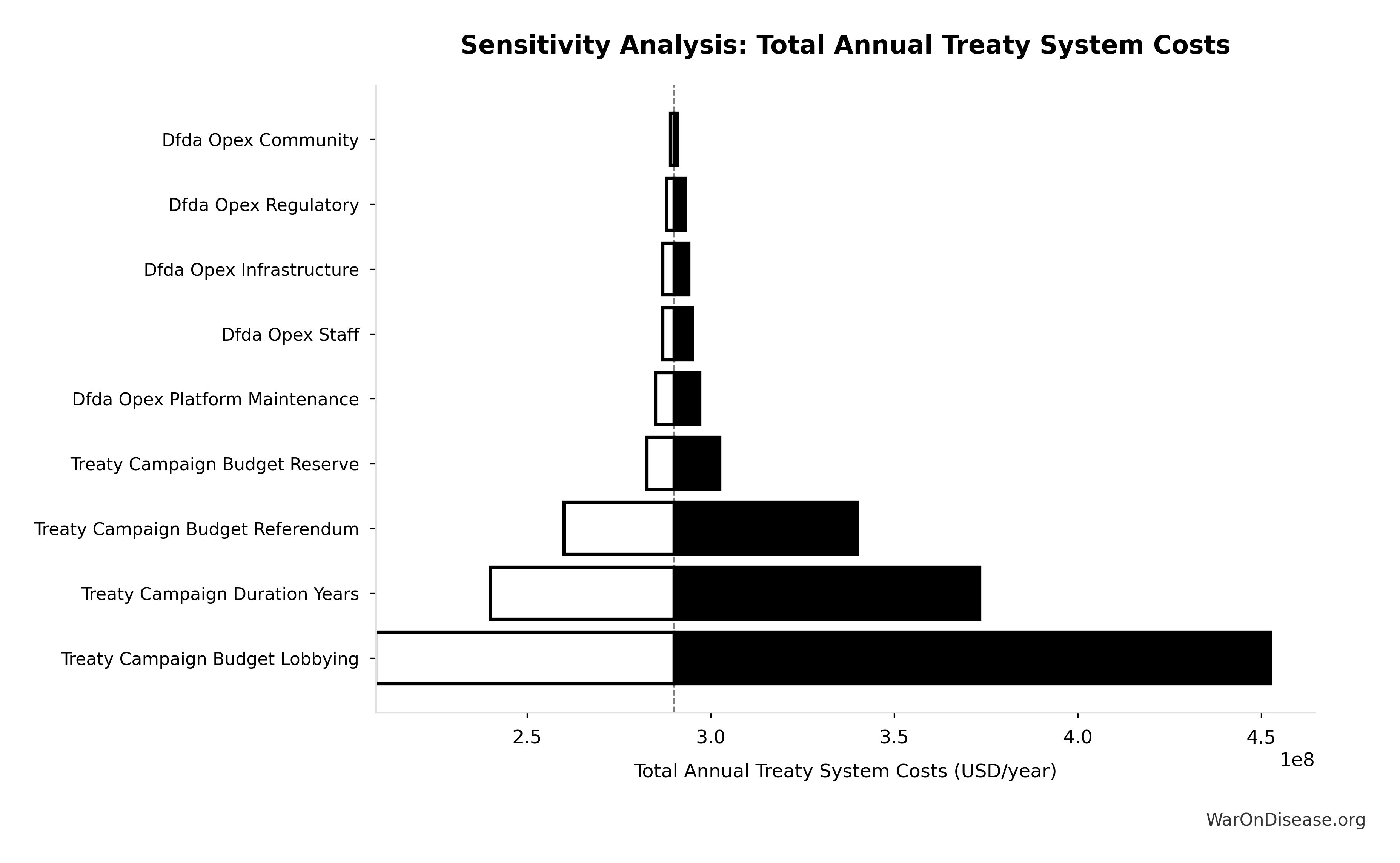
Simulation Results Summary: Unexplored Therapeutic Frontier
| Statistic | Value |
|---|---|
| Baseline (deterministic) | 99.7% |
| Mean (expected value) | 99.7% |
| Median (50th percentile) | 99.7% |
| Standard Deviation | 0.0868% |
| 90% Range (5th-95th percentile) | [99.5%, 99.8%] |
The histogram shows the distribution of Unexplored Therapeutic Frontier across 10,000 Monte Carlo simulations. The CDF (right) shows the probability of the outcome exceeding any given value, which is useful for risk assessment.
Exceedance Probability
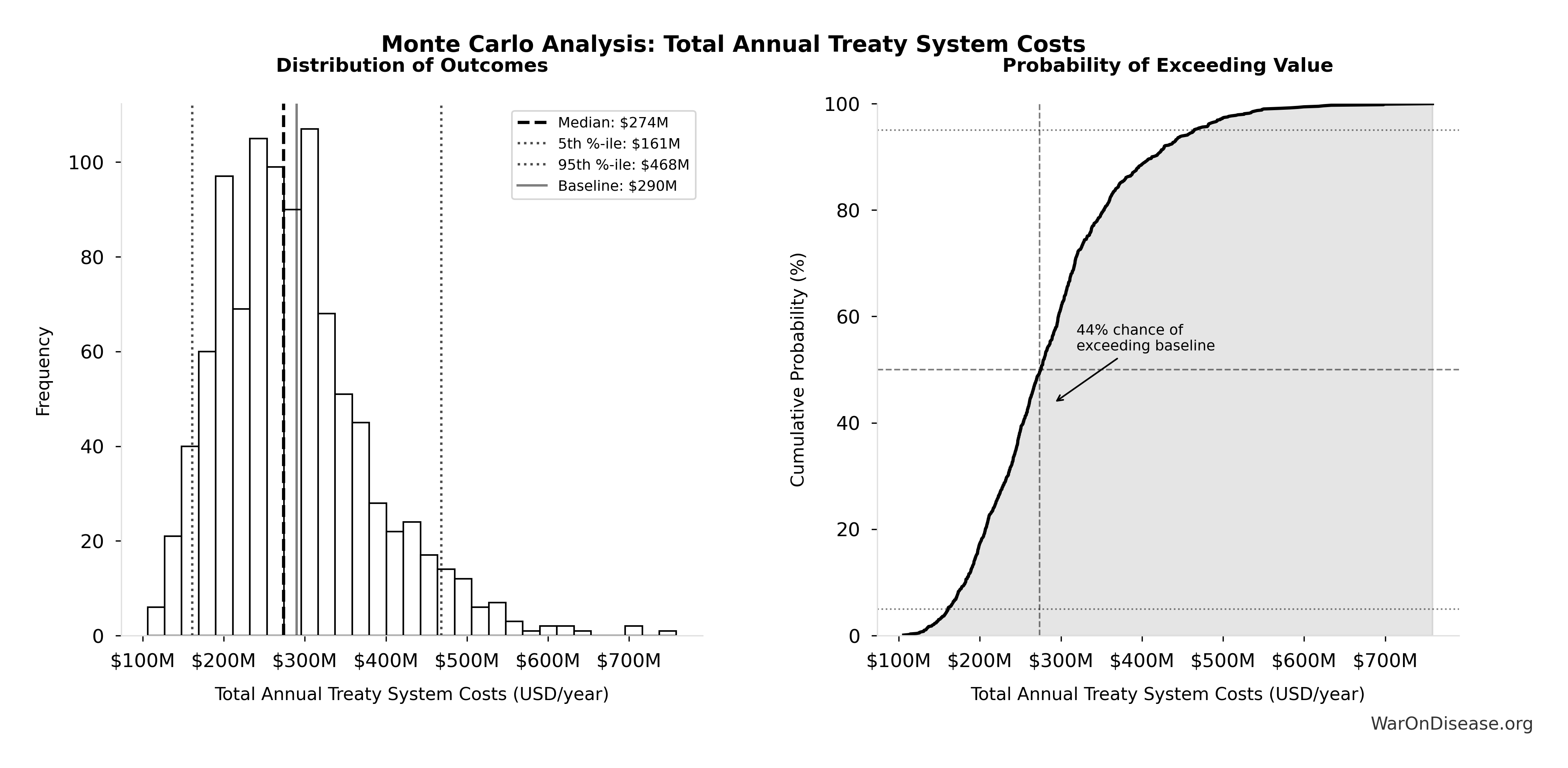
This exceedance probability chart shows the likelihood that Unexplored Therapeutic Frontier will exceed any given threshold. Higher curves indicate more favorable outcomes with greater certainty.
Annual VICTORY Incentive Alignment Bond Payout: $2.72B
Note📊 Details
Annual VICTORY Incentive Alignment Bond payout (treaty funding × bond percentage)
Inputs:
- Annual Funding from 1% of Global Military Spending Redirected to DIH 🔢: $27.2B
- Percentage of Captured Dividend Funding VICTORY Incentive Alignment Bonds: 10%
\[ \begin{gathered} Payout_{bond,ann} \\ = Funding_{treaty} \times Pct_{bond} \\ = \$27.2B \times 10\% \\ = \$2.72B \end{gathered} \] where: \[ \begin{gathered} Funding_{treaty} \\ = Spending_{mil} \times Reduce_{treaty} \\ = \$2.72T \times 1\% \\ = \$27.2B \end{gathered} \] ✓ High confidence
Annual Return Percentage for VICTORY Incentive Alignment Bondholders: 272%
Note📊 Details
Annual return percentage for VICTORY Incentive Alignment Bondholders
Inputs:
\[ \begin{gathered} r_{bond} \\ = \frac{Payout_{bond,ann}}{Cost_{campaign}} \\ = \frac{\$2.72B}{\$1B} \\ = 272\% \end{gathered} \] where: \[ \begin{gathered} Payout_{bond,ann} \\ = Funding_{treaty} \times Pct_{bond} \\ = \$27.2B \times 10\% \\ = \$2.72B \end{gathered} \] where: \[ \begin{gathered} Funding_{treaty} \\ = Spending_{mil} \times Reduce_{treaty} \\ = \$2.72T \times 1\% \\ = \$27.2B \end{gathered} \] where: \[ \begin{gathered} Cost_{campaign} \\ = Budget_{viral,base} + Budget_{lobby,treaty} \\ + Budget_{reserve} \\ = \$250M + \$650M + \$100M \\ = \$1B \end{gathered} \] ✓ High confidence
Sensitivity Analysis
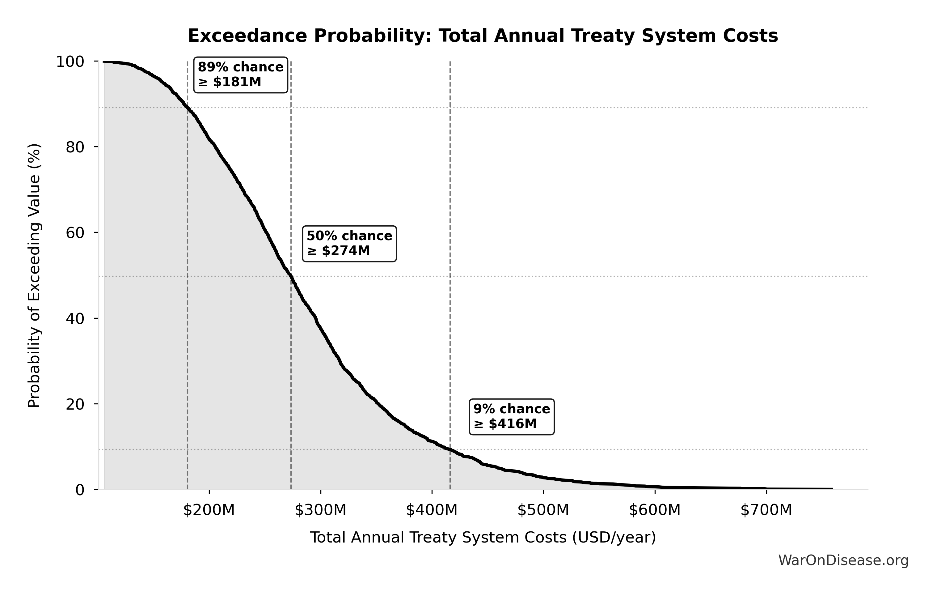
Sensitivity Indices for Annual Return Percentage for VICTORY Incentive Alignment Bondholders
Regression-based sensitivity showing which inputs explain the most variance in the output.
| Input Parameter | Sensitivity Coefficient | Interpretation |
|---|---|---|
| Total 1% Treaty Campaign Cost (USD) | -0.9366 | Strong driver |
Interpretation: Standardized coefficients show the change in output (in SD units) per 1 SD change in input. Values near ±1 indicate strong influence; values exceeding ±1 may occur with correlated inputs.
Monte Carlo Distribution

Simulation Results Summary: Annual Return Percentage for VICTORY Incentive Alignment Bondholders
| Statistic | Value |
|---|---|
| Baseline (deterministic) | 272% |
| Mean (expected value) | 293% |
| Median (50th percentile) | 287% |
| Standard Deviation | 76.3% |
| 90% Range (5th-95th percentile) | [180%, 430%] |
The histogram shows the distribution of Annual Return Percentage for VICTORY Incentive Alignment Bondholders across 10,000 Monte Carlo simulations. The CDF (right) shows the probability of the outcome exceeding any given value, which is useful for risk assessment.
Exceedance Probability
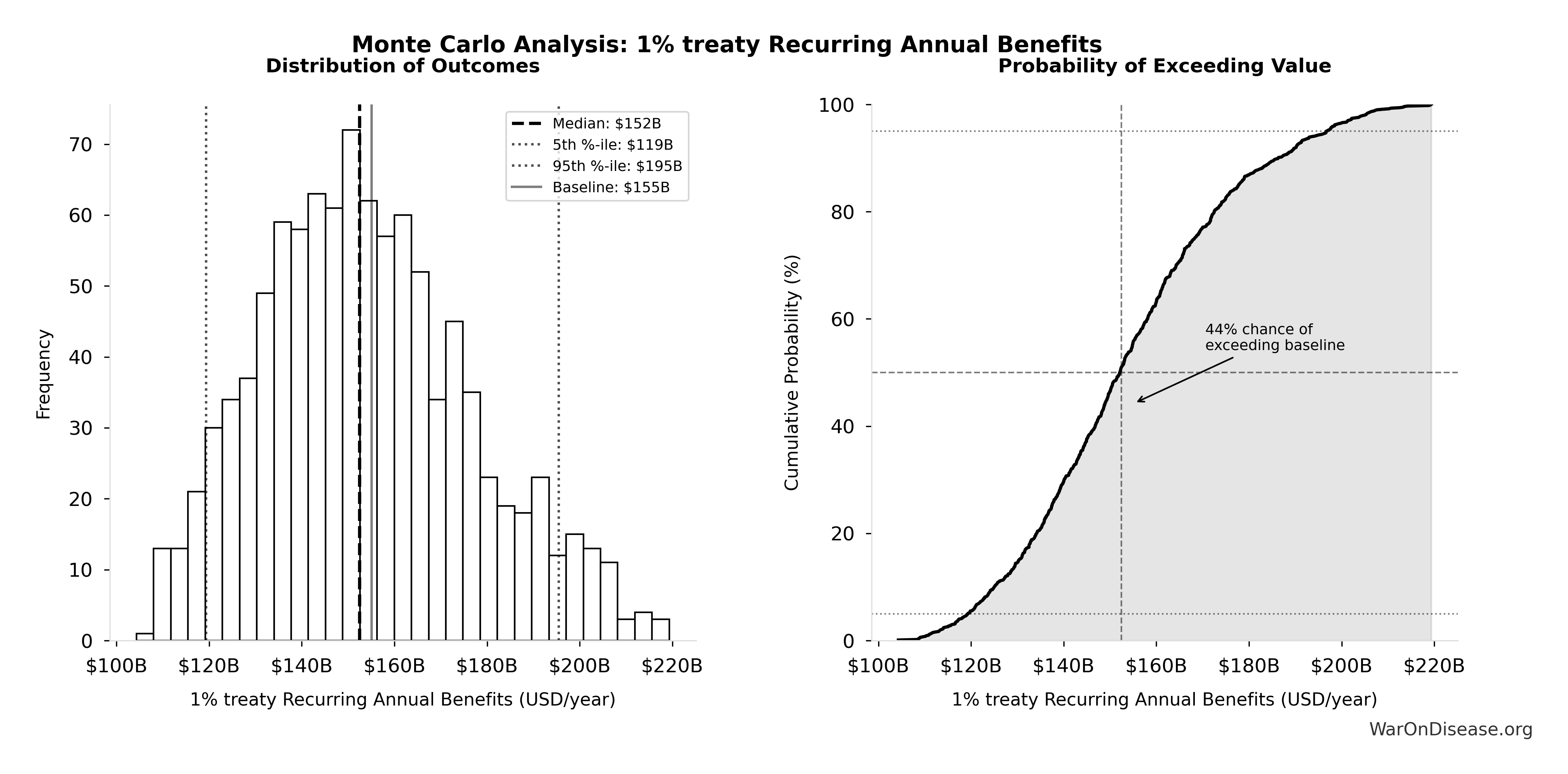
This exceedance probability chart shows the likelihood that Annual Return Percentage for VICTORY Incentive Alignment Bondholders will exceed any given threshold. Higher curves indicate more favorable outcomes with greater certainty.
Global Patients Willing to Participate in Clinical Trials: 1.08 billion people
Note📊 Details
Global chronic disease patients willing to participate in trials (2.4B × 44.8%)
Inputs:
- Global Population with Chronic Diseases 📊: 2.4 billion people (95% CI: 2 billion people - 2.8 billion people)
- Patient Willingness to Participate in Clinical Trials 📊: 44.8% (95% CI: 40% - 50%)
\[ \begin{gathered} N_{willing} \\ = N_{patients} \times Pct_{willing} \\ = 2.4B \times 44.8\% \\ = 1.08B \end{gathered} \]
~ Medium confidence
Sensitivity Analysis

Sensitivity Indices for Global Patients Willing to Participate in Clinical Trials
Regression-based sensitivity showing which inputs explain the most variance in the output.
| Input Parameter | Sensitivity Coefficient | Interpretation |
|---|---|---|
| Global Population with Chronic Diseases (people) | 1.1065 | Strong driver |
| Patient Willingness to Participate in Clinical Trials (percentage) | -0.1072 | Weak driver |
Interpretation: Standardized coefficients show the change in output (in SD units) per 1 SD change in input. Values near ±1 indicate strong influence; values exceeding ±1 may occur with correlated inputs.
Monte Carlo Distribution
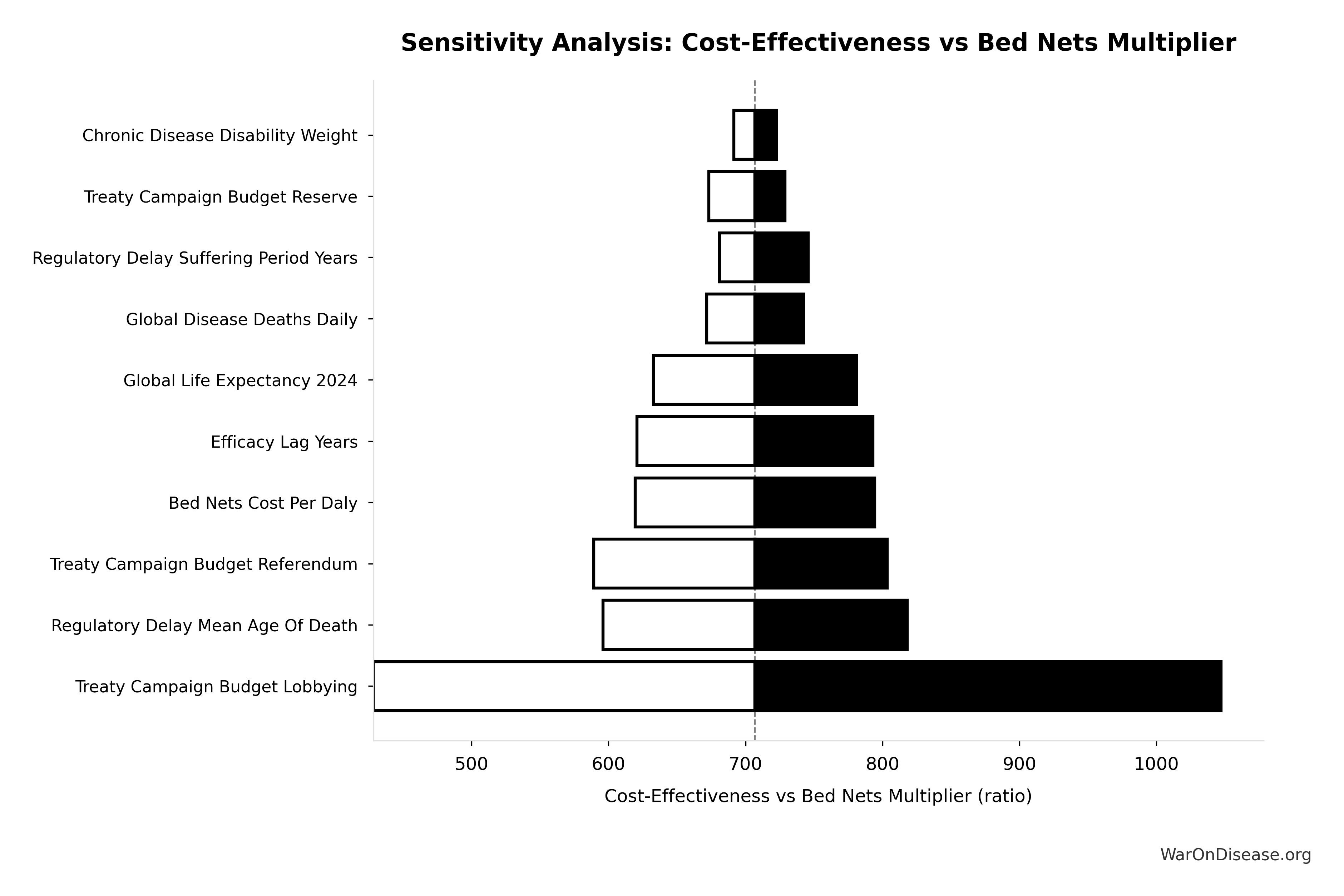
Simulation Results Summary: Global Patients Willing to Participate in Clinical Trials
| Statistic | Value |
|---|---|
| Baseline (deterministic) | 1.08 billion |
| Mean (expected value) | 1.08 billion |
| Median (50th percentile) | 1.07 billion |
| Standard Deviation | 145 million |
| 90% Range (5th-95th percentile) | [843 million, 1.34 billion] |
The histogram shows the distribution of Global Patients Willing to Participate in Clinical Trials across 10,000 Monte Carlo simulations. The CDF (right) shows the probability of the outcome exceeding any given value, which is useful for risk assessment.
Exceedance Probability
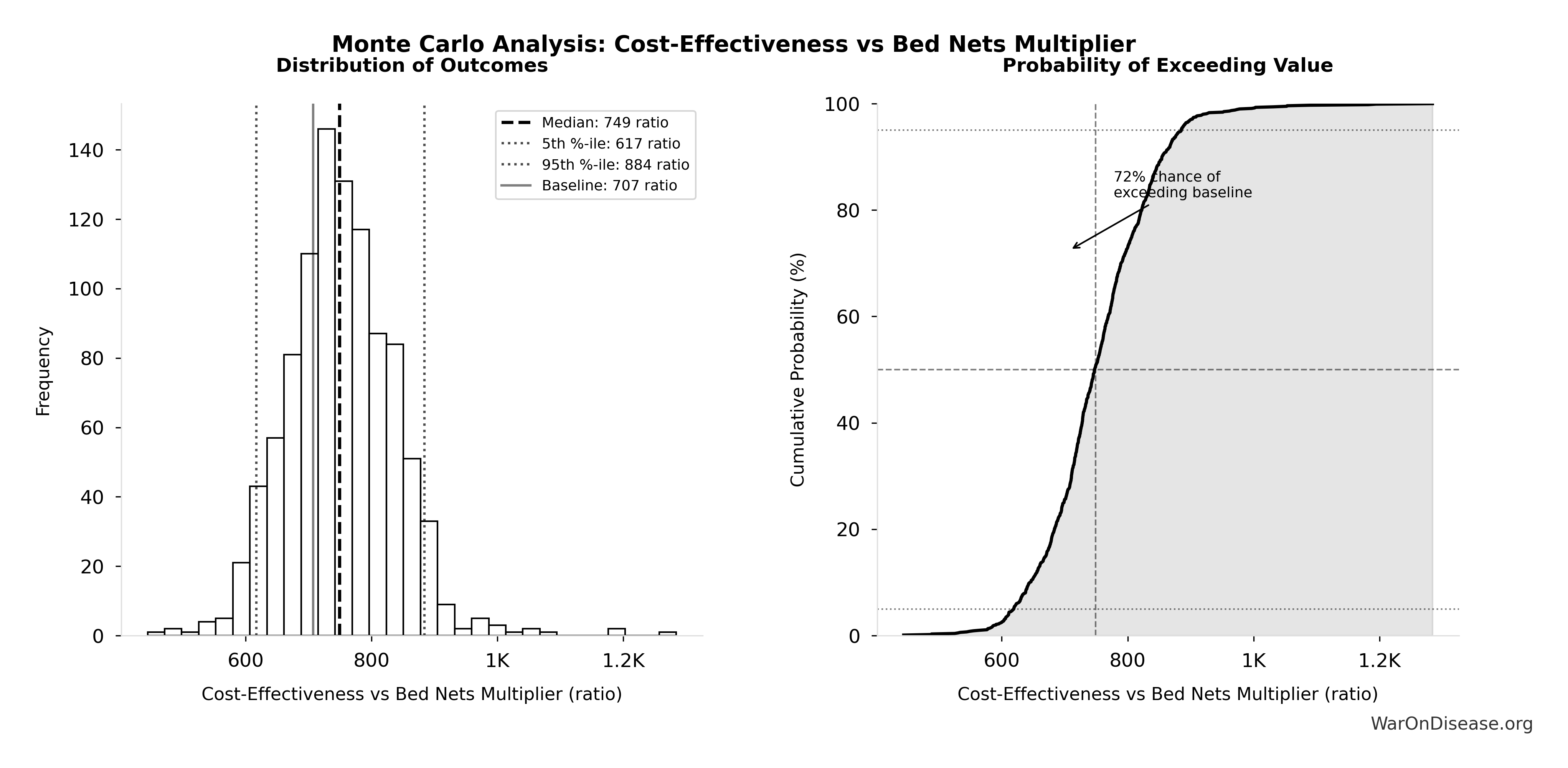
This exceedance probability chart shows the likelihood that Global Patients Willing to Participate in Clinical Trials will exceed any given threshold. Higher curves indicate more favorable outcomes with greater certainty.
Wishonia Disease Cure Fraction (20yr, Full Implementation): 100%
Note📊 Details
Wishonia disease-cure fraction over 20 years under full implementation. Uses full trial-capacity scaling and applies an upper bound of 100% of untreated disease classes.
Inputs:
- Diseases Getting First Treatment Per Year 📊: 15 diseases/year (95% CI: 8 diseases/year - 30 diseases/year)
- Trial Capacity Multiplier 🔢: 12.3x
- Wishonia Military Reallocation Physical Max Share 🔢: 87.6%
- Maximum Trial Capacity Multiplier (Physical Limit) 🔢: 566x
- Diseases Without Effective Treatment 🔢: 6.65 thousand diseases
\[ \begin{gathered} f_{cure,20,wish} \\ = \min\left(1,\frac{Treatments_{new,ann}\cdot k_{capacity,wish}\cdot 20}{D_{untreated}}\right) \end{gathered} \]
✓ High confidence
Wishonia Trajectory Average Income at Year 20: $1.16M
Note📊 Details
Average income (GDP per capita) at year 20 under the Wishonia Trajectory.
Inputs:
- Wishonia Trajectory GDP at Year 20 🔢: $10.7 quadrillion
- Global Population 2045 (Projected) 📊: 9.2 billion of people
\[ \bar{y}_{wish,20} = \frac{GDP_{wish,20}}{Pop_{2045}} \]
✓ High confidence
Sensitivity Analysis
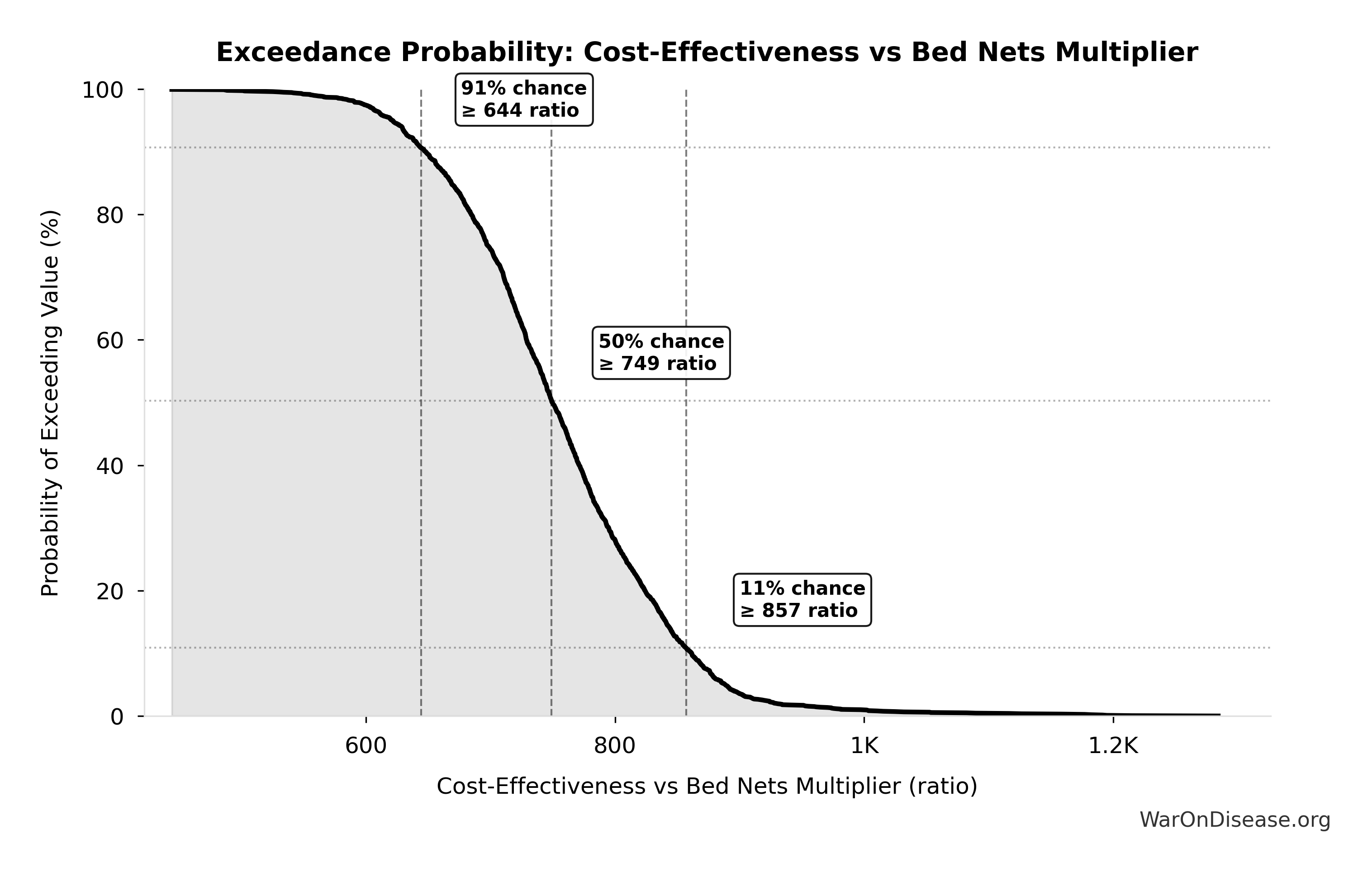
Sensitivity Indices for Wishonia Trajectory Average Income at Year 20
Regression-based sensitivity showing which inputs explain the most variance in the output.
| Input Parameter | Sensitivity Coefficient | Interpretation |
|---|---|---|
| Wishonia Trajectory GDP at Year 20 (USD) | 1.0000 | Strong driver |
Interpretation: Standardized coefficients show the change in output (in SD units) per 1 SD change in input. Values near ±1 indicate strong influence; values exceeding ±1 may occur with correlated inputs.
Monte Carlo Distribution
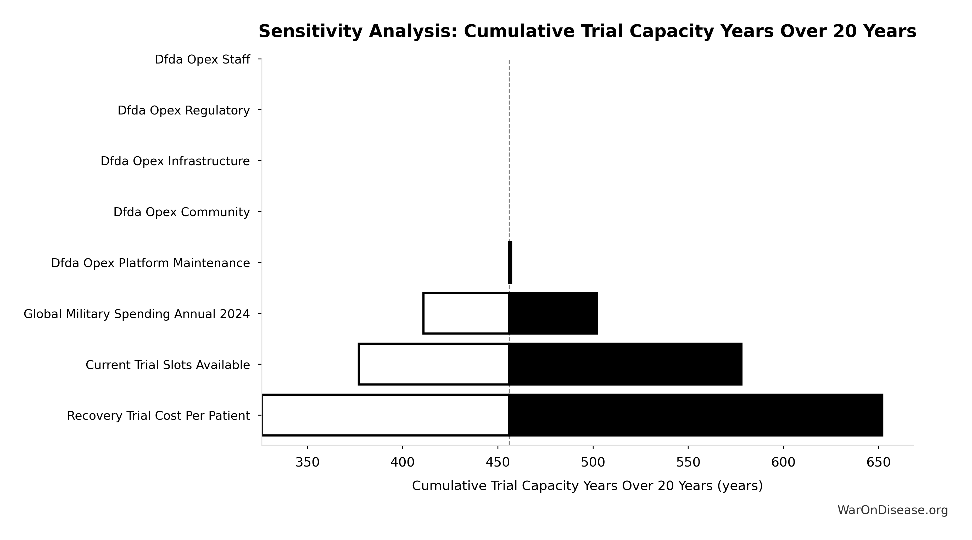
Simulation Results Summary: Wishonia Trajectory Average Income at Year 20
| Statistic | Value |
|---|---|
| Baseline (deterministic) | $1.16M |
| Mean (expected value) | $1.87M |
| Median (50th percentile) | $1.15M |
| Standard Deviation | $1.98M |
| 90% Range (5th-95th percentile) | [$395K, $6.22M] |
The histogram shows the distribution of Wishonia Trajectory Average Income at Year 20 across 10,000 Monte Carlo simulations. The CDF (right) shows the probability of the outcome exceeding any given value, which is useful for risk assessment.
Exceedance Probability
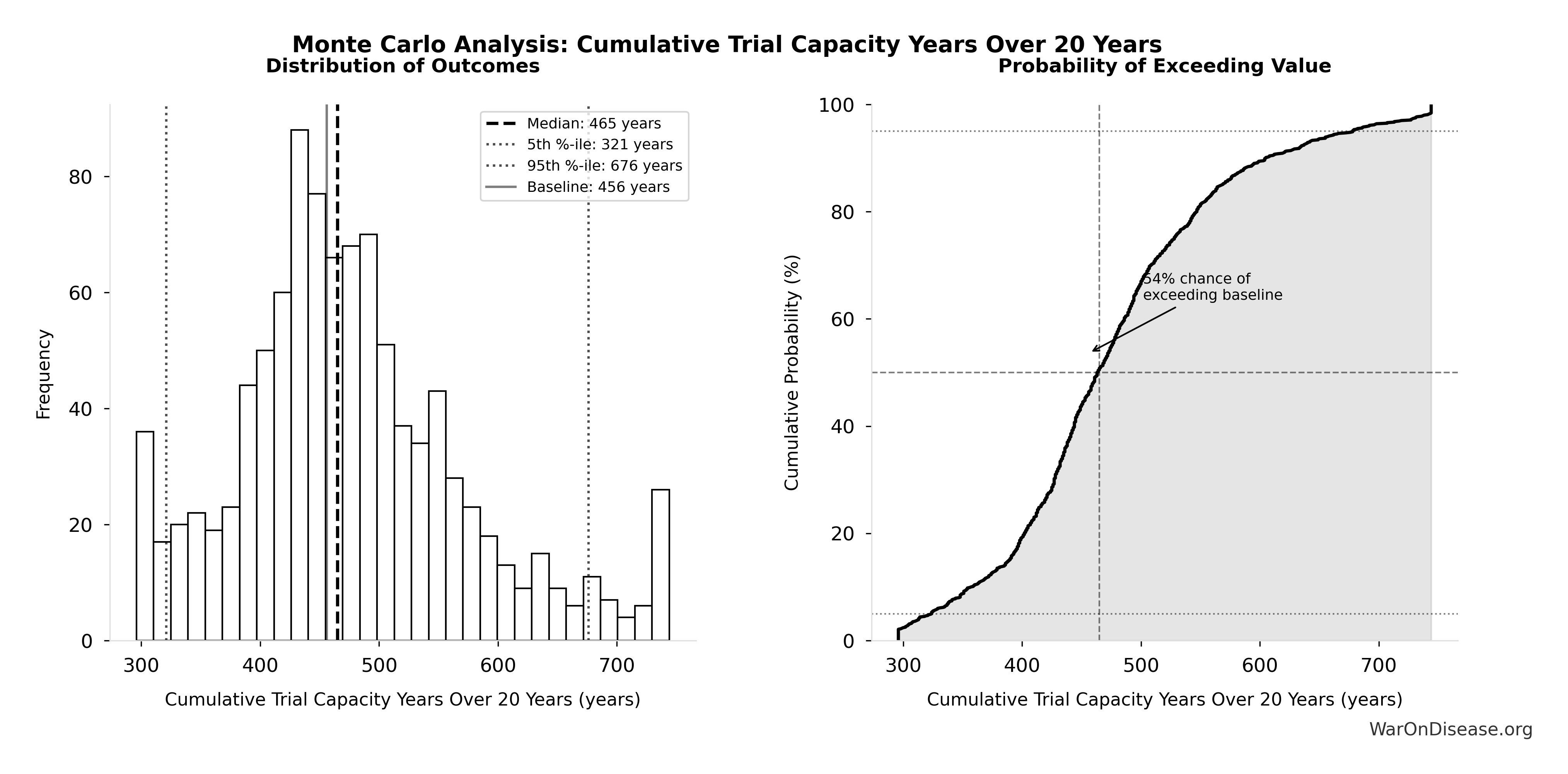
This exceedance probability chart shows the likelihood that Wishonia Trajectory Average Income at Year 20 will exceed any given threshold. Higher curves indicate more favorable outcomes with greater certainty.
Wishonia Trajectory vs Current Trajectory GDP Multiplier (Year 20): 56.7x
Note📊 Details
Wishonia Trajectory GDP at year 20 as a multiple of current trajectory GDP at year 20.
Inputs:
- Wishonia Trajectory GDP at Year 20 🔢: $10.7 quadrillion
- Current Trajectory GDP at Year 20 🔢: $188T
\[ \begin{gathered} k_{wish:base,20} \\ = \frac{GDP_{wish,20}}{GDP_{base,20}} \\ = \frac{\$10700T}{\$188T} \\ = 56.7 \end{gathered} \] where: \[ GDP_{wish,20}=GDP_0(1+g_{ramp})^3(1+g_{full})^{17} \] where: \[ s_{mil,max} = Cut_{WW2} = 87.6\% = 87.6\% \] where: \[ \begin{gathered} Cut_{WW2} \\ = 1 - \frac{Spending_{US,1947}}{Spending_{US,1945}} \\ = 1 - \frac{\$176B}{\$1.42T} \\ = 87.6\% \end{gathered} \] where: \[ \begin{gathered} f_{cure,20,wish} \\ = \min\left(1,\frac{Treatments_{new,ann}\cdot k_{capacity,wish}\cdot 20}{D_{untreated}}\right) \end{gathered} \] where: \[ \begin{gathered} k_{capacity} \\ = \frac{N_{fundable,dFDA}}{Slots_{curr}} \\ = \frac{23.4M}{1.9M} \\ = 12.3 \end{gathered} \] where: \[ \begin{gathered} N_{fundable,dFDA} \\ = \frac{Subsidies_{dFDA,ann}}{Cost_{pragmatic,pt}} \\ = \frac{\$21.8B}{\$929} \\ = 23.4M \end{gathered} \] where: \[ \begin{gathered} Subsidies_{dFDA,ann} \\ = Funding_{dFDA,ann} - OPEX_{dFDA} \\ = \$21.8B - \$40M \\ = \$21.8B \end{gathered} \] where: \[ \begin{gathered} OPEX_{dFDA} \\ = Cost_{platform} + Cost_{staff} + Cost_{infra} \\ + Cost_{regulatory} + Cost_{community} \\ = \$15M + \$10M + \$8M + \$5M + \$2M \\ = \$40M \end{gathered} \] where: \[ \begin{gathered} k_{capacity,max} \\ = \frac{N_{willing}}{Slots_{curr}} \\ = \frac{1.08B}{1.9M} \\ = 566 \end{gathered} \] where: \[ \begin{gathered} N_{willing} \\ = N_{patients} \times Pct_{willing} \\ = 2.4B \times 44.8\% \\ = 1.08B \end{gathered} \] where: \[ \begin{gathered} N_{untreated} \\ = N_{rare} \times 0.95 \\ = 7{,}000 \times 0.95 \\ = 6{,}650 \end{gathered} \] where: \[ GDP_{base,20} = GDP_0(1+g_{base})^{20} \] ✓ High confidence
Sensitivity Analysis
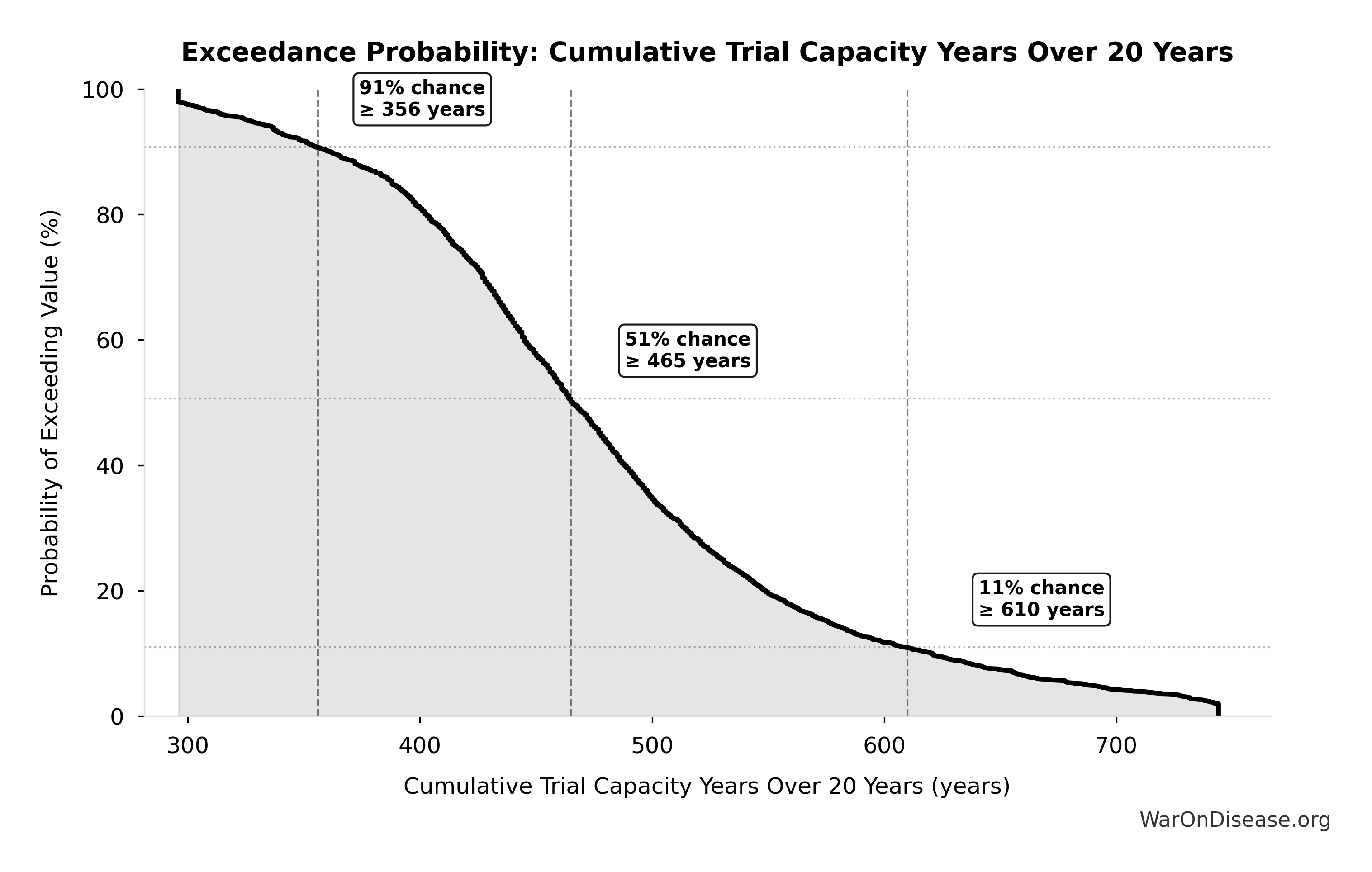
Sensitivity Indices for Wishonia Trajectory vs Current Trajectory GDP Multiplier (Year 20)
Regression-based sensitivity showing which inputs explain the most variance in the output.
| Input Parameter | Sensitivity Coefficient | Interpretation |
|---|---|---|
| Wishonia Trajectory GDP at Year 20 (USD) | 1.0000 | Strong driver |
| Current Trajectory GDP at Year 20 (USD) | 0.0000 | Minimal effect |
Interpretation: Standardized coefficients show the change in output (in SD units) per 1 SD change in input. Values near ±1 indicate strong influence; values exceeding ±1 may occur with correlated inputs.
Monte Carlo Distribution
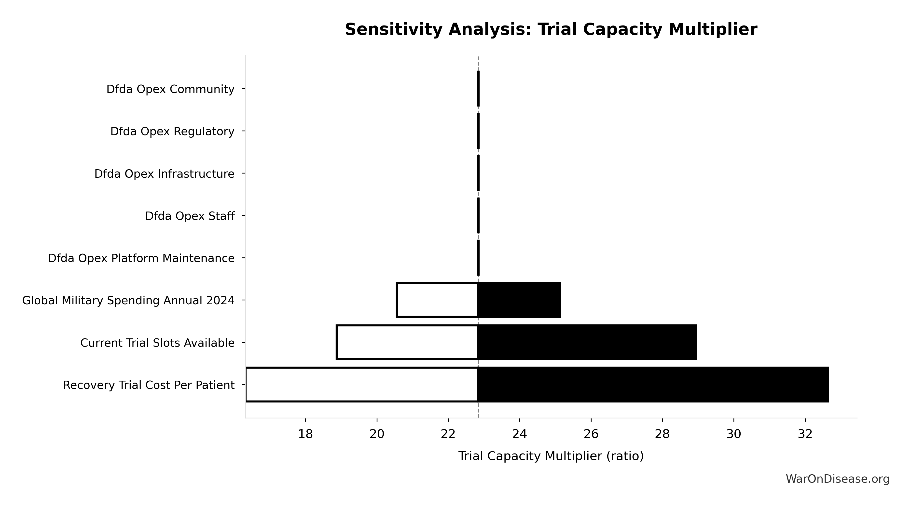
Simulation Results Summary: Wishonia Trajectory vs Current Trajectory GDP Multiplier (Year 20)
| Statistic | Value |
|---|---|
| Baseline (deterministic) | 56.7x |
| Mean (expected value) | 91.5x |
| Median (50th percentile) | 56.2x |
| Standard Deviation | 96.6x |
| 90% Range (5th-95th percentile) | [19.3x, 304x] |
The histogram shows the distribution of Wishonia Trajectory vs Current Trajectory GDP Multiplier (Year 20) across 10,000 Monte Carlo simulations. The CDF (right) shows the probability of the outcome exceeding any given value, which is useful for risk assessment.
Exceedance Probability
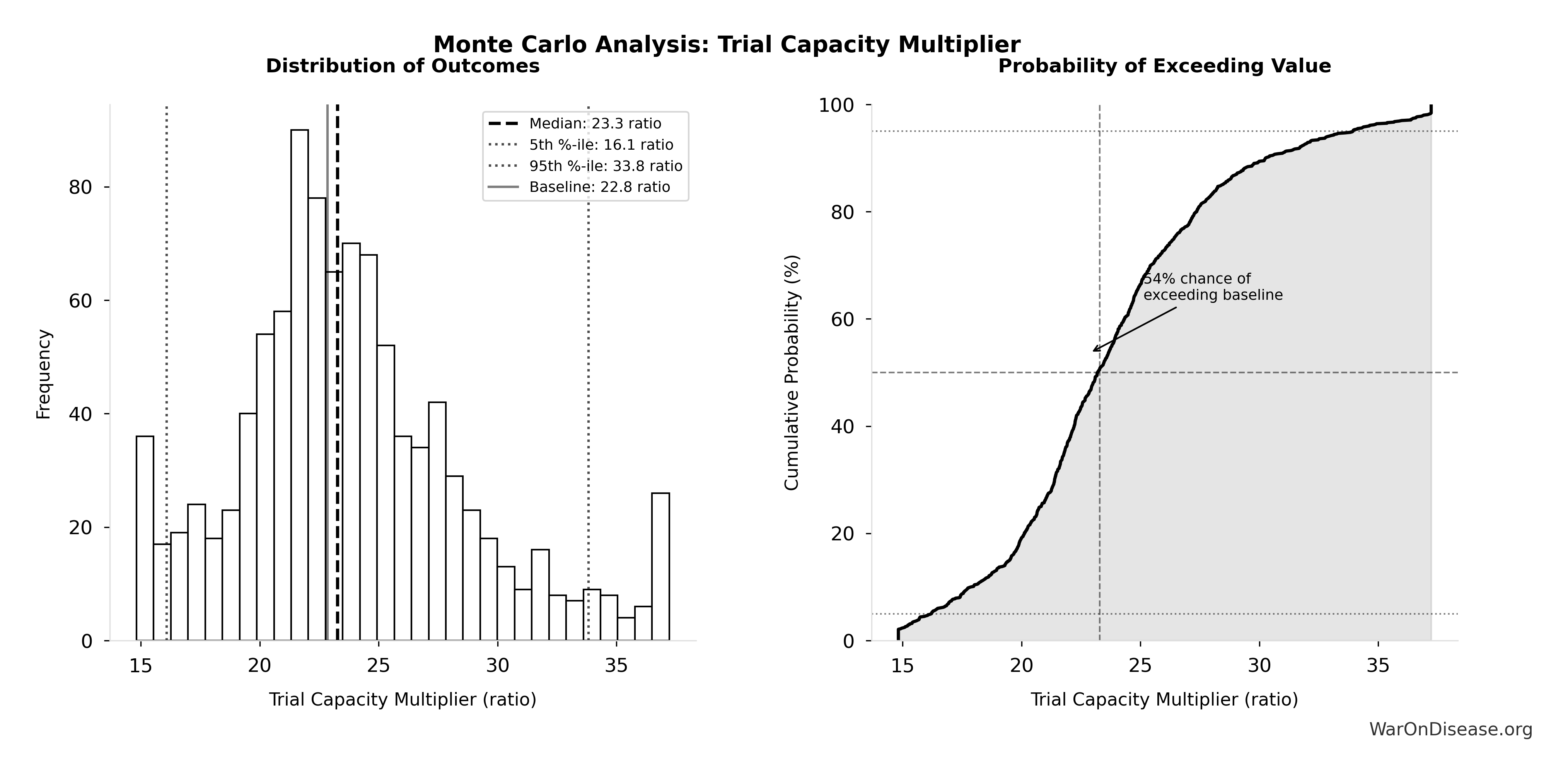
This exceedance probability chart shows the likelihood that Wishonia Trajectory vs Current Trajectory GDP Multiplier (Year 20) will exceed any given threshold. Higher curves indicate more favorable outcomes with greater certainty.
Wishonia Trajectory GDP at Year 20: $10.7 quadrillion
Note📊 Details
Projected global GDP at year 20 under the Wishonia Trajectory. Model applies all Wishonia policy channels and redirects the full Political Dysfunction Tax non-health opportunity pool to highest-marginal-value uses. Health recovery is modeled separately through disease burden removal to avoid overlap. Military and non-health reallocation effects are ramped at 50% intensity for the first 3 years, then 100% for years 4-20, reflecting implementation lag. Military reallocation uses a physically demonstrated upper bound (post-WW2 demobilization) rather than an arbitrary policy cap.
Inputs:
- Global GDP (2025) 📊: $115T
- Baseline Global GDP Growth Rate: 2.5%
- Wishonia Military Reallocation Physical Max Share 🔢: 87.6%
- GDP Growth Boost at 30% Military Reallocation: 5.5% (95% CI: 3.5% - 7.5%)
- R&D Spillover Multiplier: 2x (95% CI: 1.5x - 2.5x)
- Wishonia Disease Cure Fraction (20yr, Full Implementation) 🔢: 100%
- Disease Burden as % of GDP 📊: 13%
- Global Science Opportunity Cost 📊: $4T (95% CI: $2T - $10T)
- Global Lead Poisoning Cost 📊: $6T (95% CI: $4T - $8T)
- Global Migration Opportunity Cost 📊: $57T (95% CI: $57T - $170T)
- Economic Multiplier for Healthcare Investment 📊: 4.3x (95% CI: 3x - 6x)
- Economic Multiplier for Military Spending 📊: 0.6x (95% CI: 0.4x - 0.9x)
\[ GDP_{wish,20}=GDP_0(1+g_{ramp})^3(1+g_{full})^{17} \]
✓ High confidence
Sensitivity Analysis
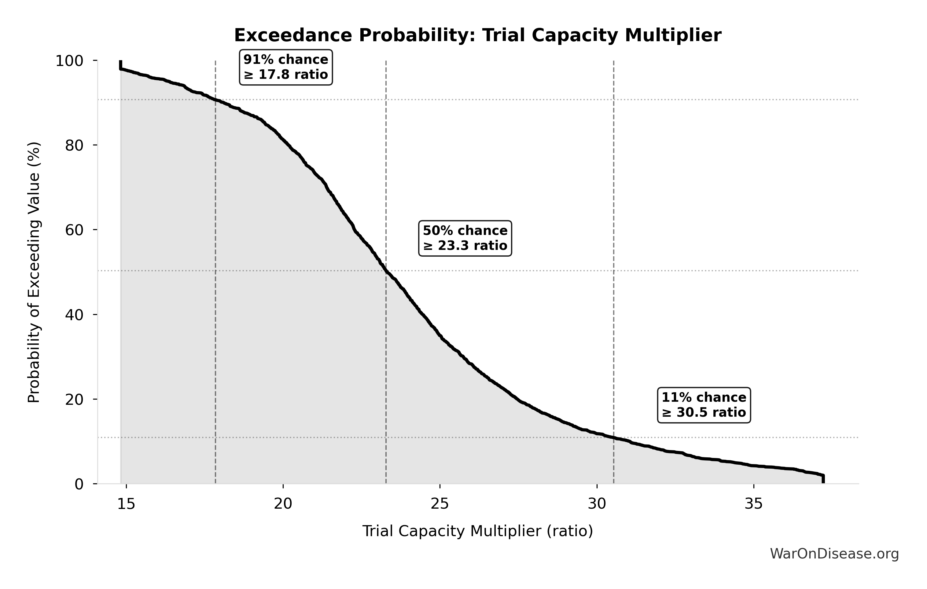
Sensitivity Indices for Wishonia Trajectory GDP at Year 20
Regression-based sensitivity showing which inputs explain the most variance in the output.
| Input Parameter | Sensitivity Coefficient | Interpretation |
|---|---|---|
| Economic Multiplier for Healthcare Investment (x) | -1.7151 | Strong driver |
| R&D Spillover Multiplier (x) | 1.3750 | Strong driver |
| Global Science Opportunity Cost (USD) | 0.9398 | Strong driver |
| Global Migration Opportunity Cost (USD) | 0.6829 | Strong driver |
| GDP Growth Boost at 30% Military Reallocation (rate) | -0.3425 | Moderate driver |
| Global Lead Poisoning Cost (USD) | 0.2431 | Weak driver |
| Economic Multiplier for Military Spending (x) | -0.1554 | Weak driver |
Interpretation: Standardized coefficients show the change in output (in SD units) per 1 SD change in input. Values near ±1 indicate strong influence; values exceeding ±1 may occur with correlated inputs.
Monte Carlo Distribution
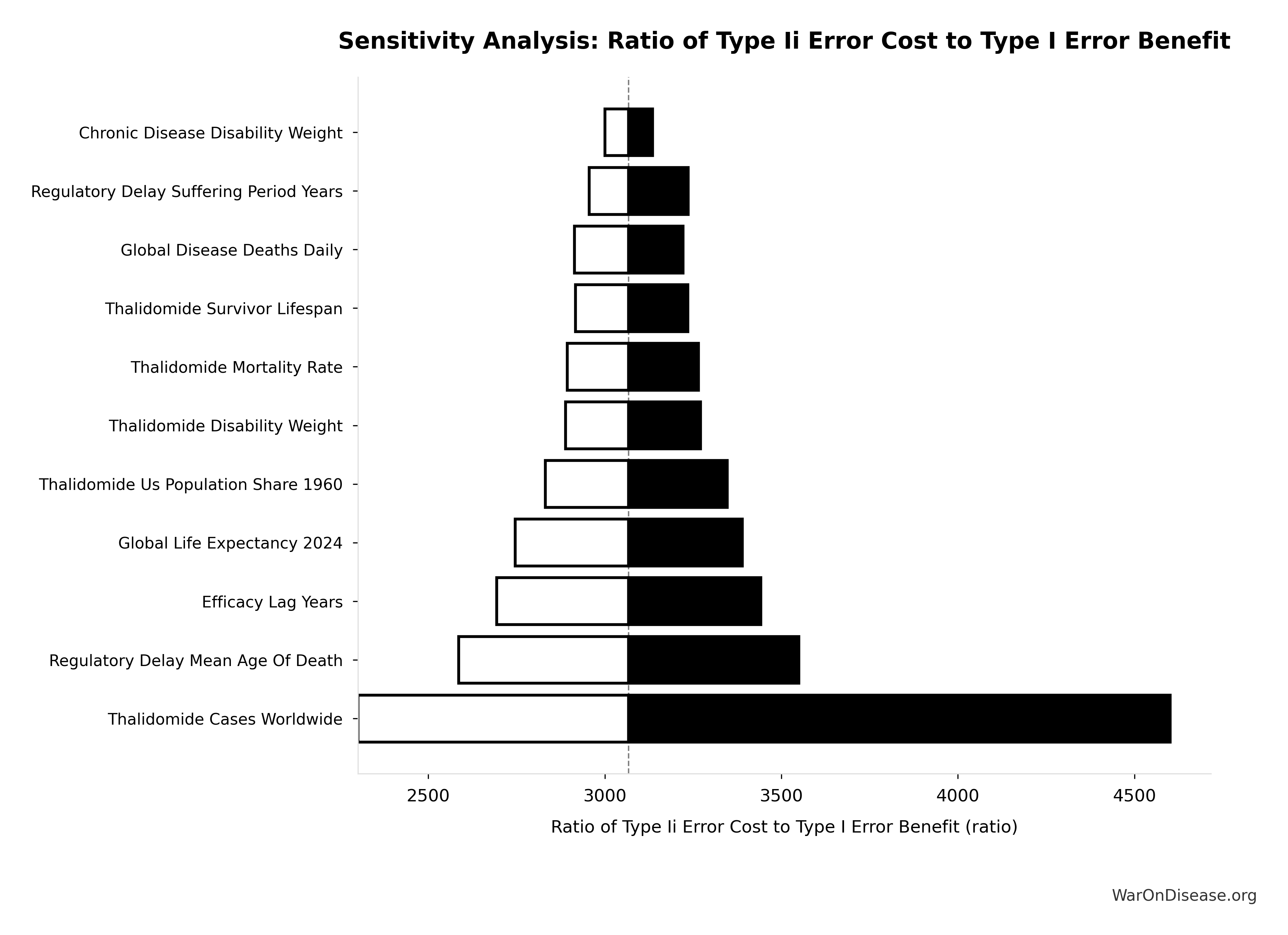
Simulation Results Summary: Wishonia Trajectory GDP at Year 20
| Statistic | Value |
|---|---|
| Baseline (deterministic) | $10.7 quadrillion |
| Mean (expected value) | $17.2 quadrillion |
| Median (50th percentile) | $10.6 quadrillion |
| Standard Deviation | $18.2 quadrillion |
| 90% Range (5th-95th percentile) | [$3.64 quadrillion, $57.2 quadrillion] |
The histogram shows the distribution of Wishonia Trajectory GDP at Year 20 across 10,000 Monte Carlo simulations. The CDF (right) shows the probability of the outcome exceeding any given value, which is useful for risk assessment.
Exceedance Probability
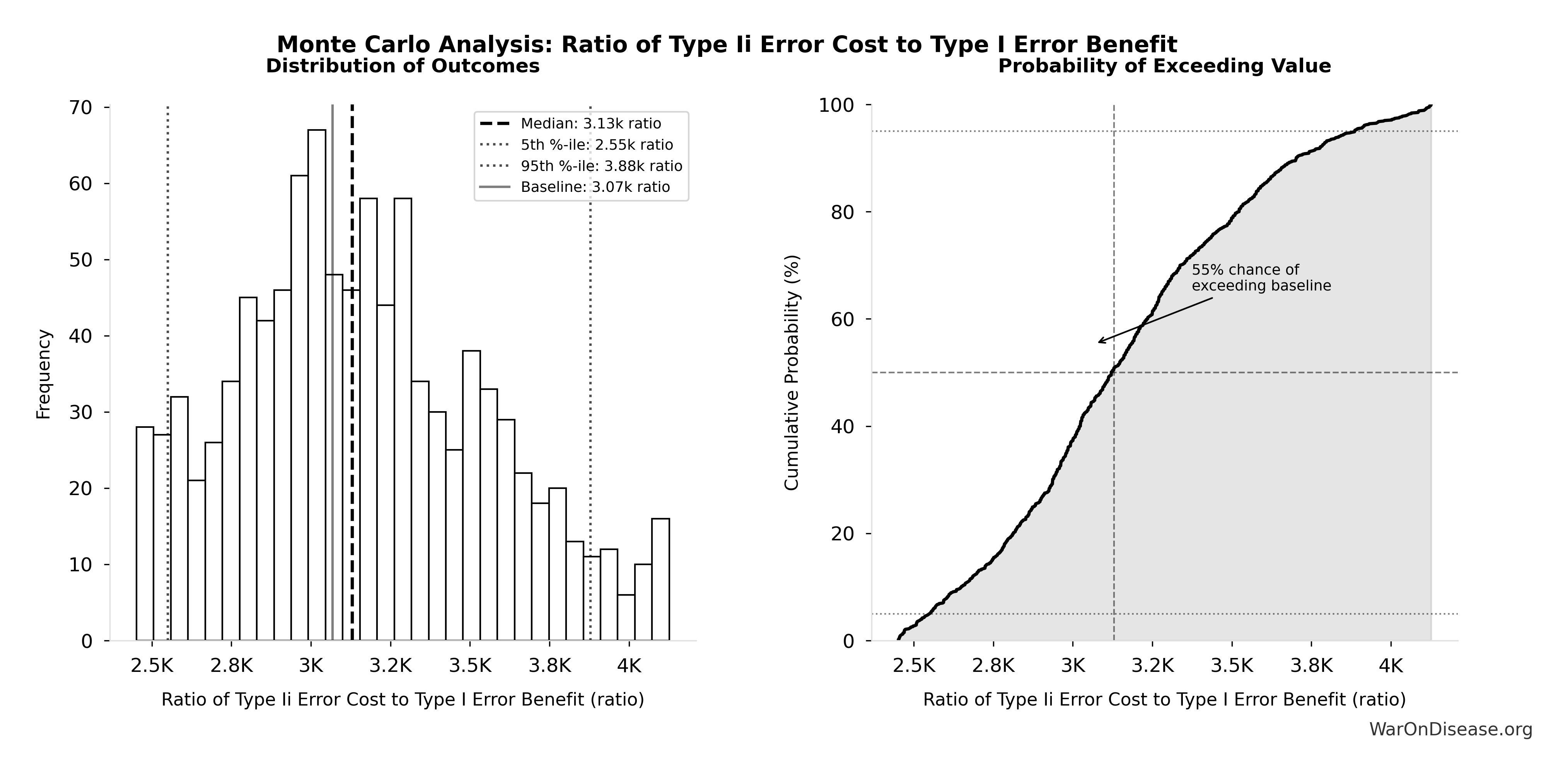
This exceedance probability chart shows the likelihood that Wishonia Trajectory GDP at Year 20 will exceed any given threshold. Higher curves indicate more favorable outcomes with greater certainty.
External Data Sources
Parameters sourced from peer-reviewed publications, institutional databases, and authoritative reports.
ADAPTABLE Trial Cost per Patient: $929
Note📊 Details
Cost per patient in ADAPTABLE trial ($14M PCORI grant / 15,076 patients). Note: This is the direct grant cost; true cost including in-kind may be 10-40% higher.
Source:1
Uncertainty Range
Technical: 95% CI: [$929, $1.4K] • Distribution: Lognormal
What this means: There’s significant uncertainty here. The true value likely falls between $929 and $1.4K (±25%). This represents a wide range that our Monte Carlo simulations account for when calculating overall uncertainty in the results.
The lognormal distribution means values can’t go negative and have a longer tail toward higher values (common for costs and populations).
Input Distribution
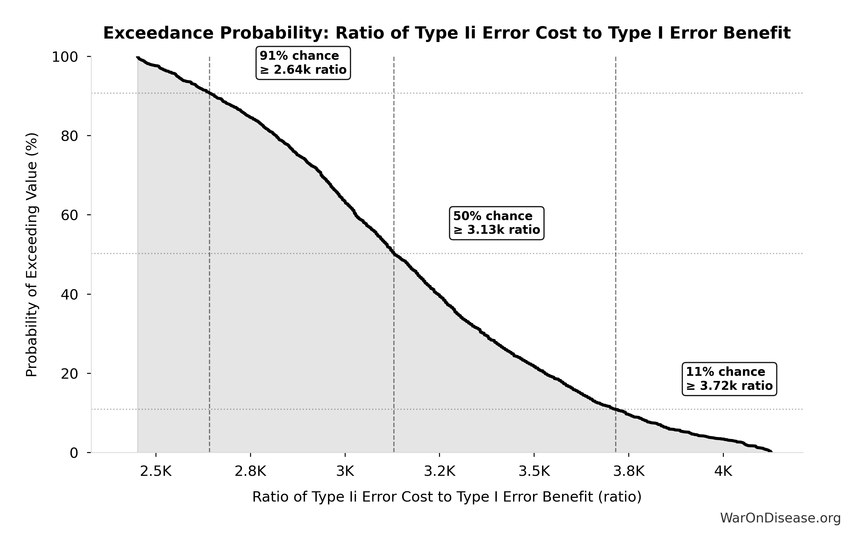
This chart shows the assumed probability distribution for this parameter. The shaded region represents the 95% confidence interval where we expect the true value to fall.
~ Medium confidence
ADAPTABLE Trial Total Cost: $14M
Note📊 Details
PCORI grant for ADAPTABLE trial (2016-2019). Note: Direct funding only; total costs including site overhead and in-kind contributions from health systems may be higher.
Source:1
Uncertainty Range
Technical: 95% CI: [$14M, $20M] • Distribution: Lognormal
What this means: This estimate has moderate uncertainty. The true value likely falls between $14M and $20M (±21%). This represents a reasonable range that our Monte Carlo simulations account for when calculating overall uncertainty in the results.
The lognormal distribution means values can’t go negative and have a longer tail toward higher values (common for costs and populations).
Input Distribution
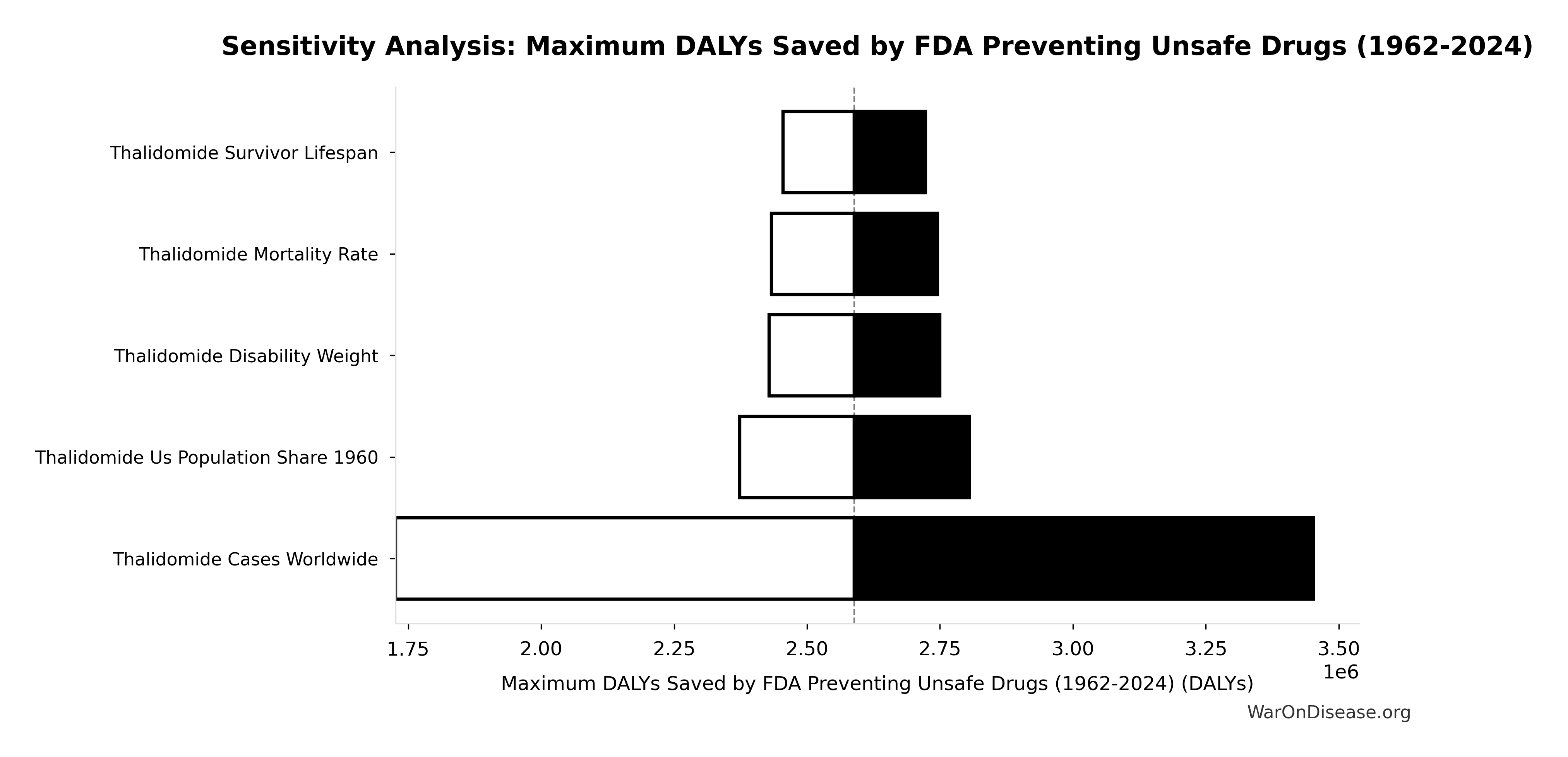
This chart shows the assumed probability distribution for this parameter. The shaded region represents the 95% confidence interval where we expect the true value to fall.
~ Medium confidence
Antidepressant Trial Exclusion Rate: 86.1%
Note📊 Details
Mean exclusion rate in antidepressant trials (86.1% of real-world patients excluded)
Source:2
✓ High confidence
Average Annual Stock Market Return: 10%
Note📊 Details
Bed Nets Cost per DALY: $89
Note📊 Details
GiveWell cost per DALY for insecticide-treated bed nets (midpoint estimate, range $78-100). DALYs (Disability-Adjusted Life Years) measure disease burden by combining years of life lost and years lived with disability. Bed nets prevent malaria deaths and are considered a gold standard benchmark for cost-effective global health interventions - if an intervention costs less per DALY than bed nets, it’s exceptionally cost-effective. GiveWell synthesizes peer-reviewed academic research with transparent, rigorous methodology and extensive external expert review.
Source:5
Uncertainty Range
Technical: 95% CI: [$78, $100] • Distribution: Normal
What this means: This estimate has moderate uncertainty. The true value likely falls between $78 and $100 (±12%). This represents a reasonable range that our Monte Carlo simulations account for when calculating overall uncertainty in the results.
The normal distribution means values cluster around the center with equal chances of being higher or lower.
Input Distribution
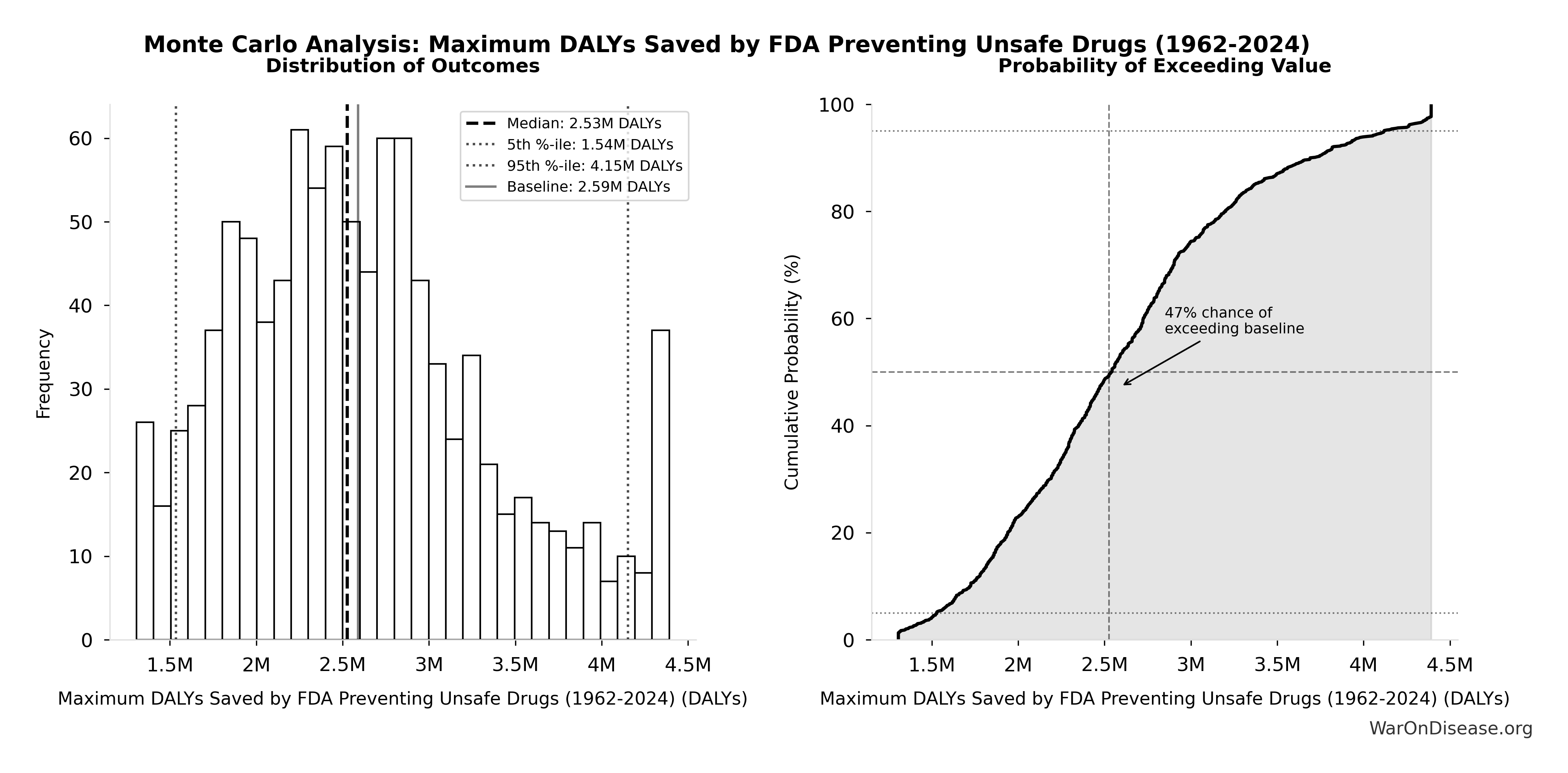
This chart shows the assumed probability distribution for this parameter. The shaded region represents the 95% confidence interval where we expect the true value to fall.
✓ High confidence • 📊 Peer-reviewed
Estimated Annual Global Economic Benefit from Childhood Vaccination Programs: $15B
Note📊 Details
Estimated annual global economic benefit from childhood vaccination programs (measles, polio, etc.)
Source:8
Uncertainty Range
Technical: Distribution: Lognormal (SE: $4.5B)
Input Distribution
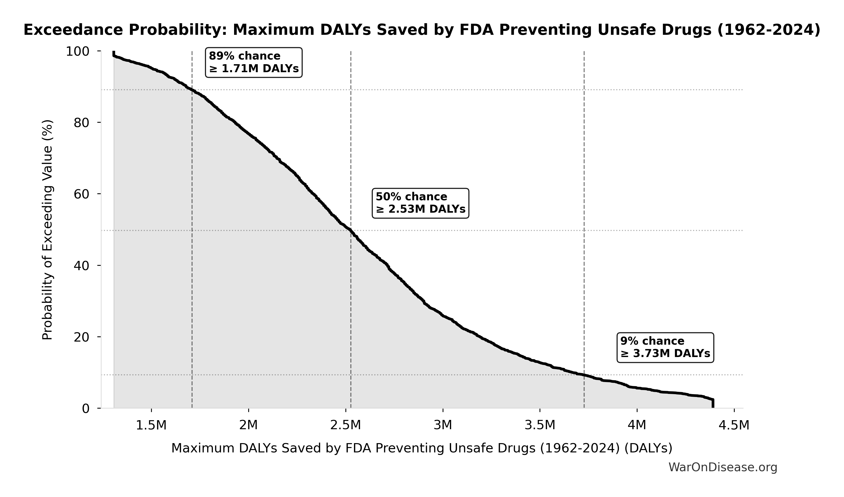
This chart shows the assumed probability distribution for this parameter. The shaded region represents the 95% confidence interval where we expect the true value to fall.
✓ High confidence
Return on Investment from Childhood Vaccination Programs: 13:1
Note📊 Details
Disability Weight for Untreated Chronic Conditions: 0.35 weight
Note📊 Details
Disability weight for untreated chronic conditions (WHO Global Burden of Disease)
Source:4
Uncertainty Range
Technical: Distribution: Normal (SE: 0.07 weight)
Input Distribution
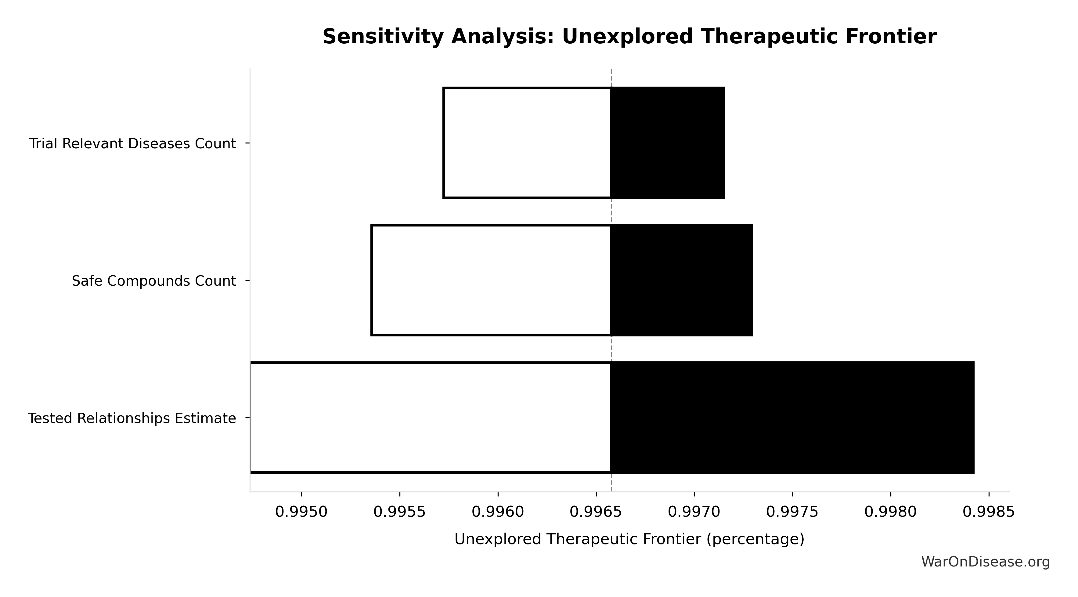
This chart shows the assumed probability distribution for this parameter. The shaded region represents the 95% confidence interval where we expect the true value to fall.
~ Medium confidence • 📊 Peer-reviewed
Current Active Trials at Any Given Time: 10 thousand trials
Note📊 Details
Current Clinical Trial Participation Rate: 0.06%
Note📊 Details
Global Population with Chronic Diseases: 2.4 billion people
Note📊 Details
Global population with chronic diseases
Source:14
Uncertainty Range
Technical: 95% CI: [2 billion people, 2.8 billion people] • Distribution: Lognormal
What this means: This estimate has moderate uncertainty. The true value likely falls between 2 billion people and 2.8 billion people (±17%). This represents a reasonable range that our Monte Carlo simulations account for when calculating overall uncertainty in the results.
The lognormal distribution means values can’t go negative and have a longer tail toward higher values (common for costs and populations).
Input Distribution

This chart shows the assumed probability distribution for this parameter. The shaded region represents the 95% confidence interval where we expect the true value to fall.
✓ High confidence
Average Annual New Drug Approvals Globally: 50 drugs/year
Note📊 Details
Average annual new drug approvals globally
Source:15
Uncertainty Range
Technical: 95% CI: [45 drugs/year, 60 drugs/year] • Distribution: Lognormal
What this means: This estimate has moderate uncertainty. The true value likely falls between 45 drugs/year and 60 drugs/year (±15%). This represents a reasonable range that our Monte Carlo simulations account for when calculating overall uncertainty in the results.
The lognormal distribution means values can’t go negative and have a longer tail toward higher values (common for costs and populations).
Input Distribution
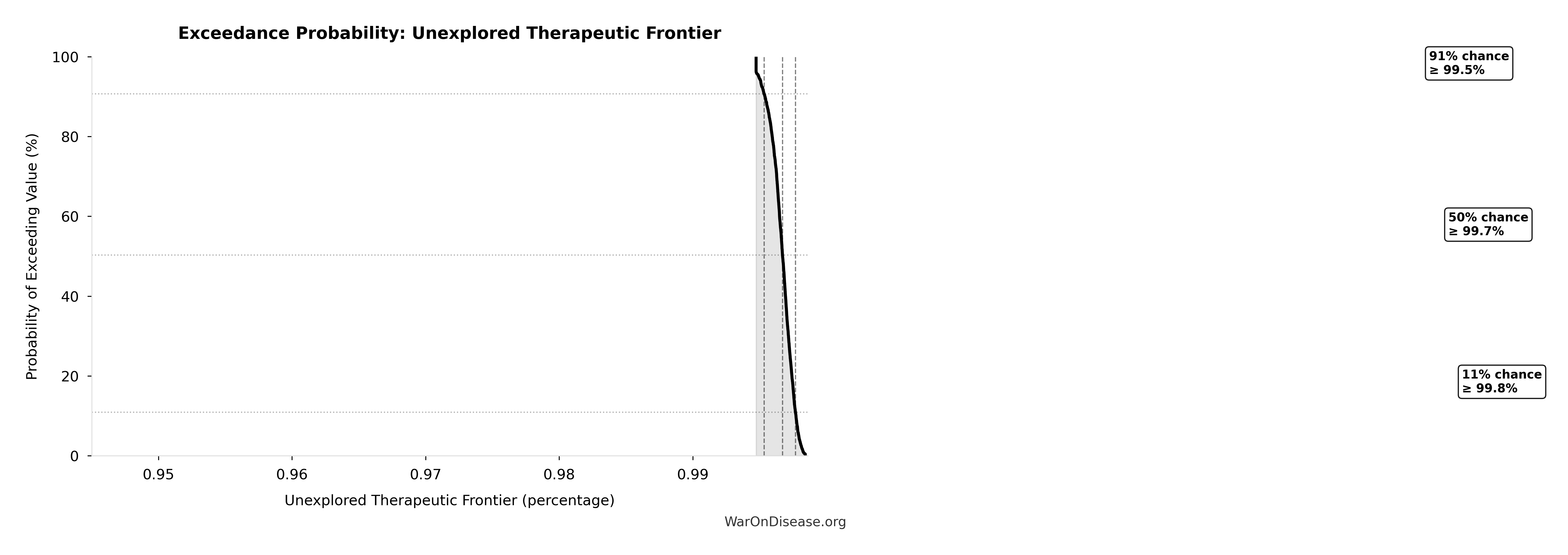
This chart shows the assumed probability distribution for this parameter. The shaded region represents the 95% confidence interval where we expect the true value to fall.
✓ High confidence
Current Global Clinical Trials per Year: 3.3 thousand trials/year
Note📊 Details
Current global clinical trials per year
Source:18
Uncertainty Range
Technical: 95% CI: [2.64 thousand trials/year, 3.96 thousand trials/year] • Distribution: Lognormal
What this means: This estimate has moderate uncertainty. The true value likely falls between 2.64 thousand trials/year and 3.96 thousand trials/year (±20%). This represents a reasonable range that our Monte Carlo simulations account for when calculating overall uncertainty in the results.
The lognormal distribution means values can’t go negative and have a longer tail toward higher values (common for costs and populations).
Input Distribution
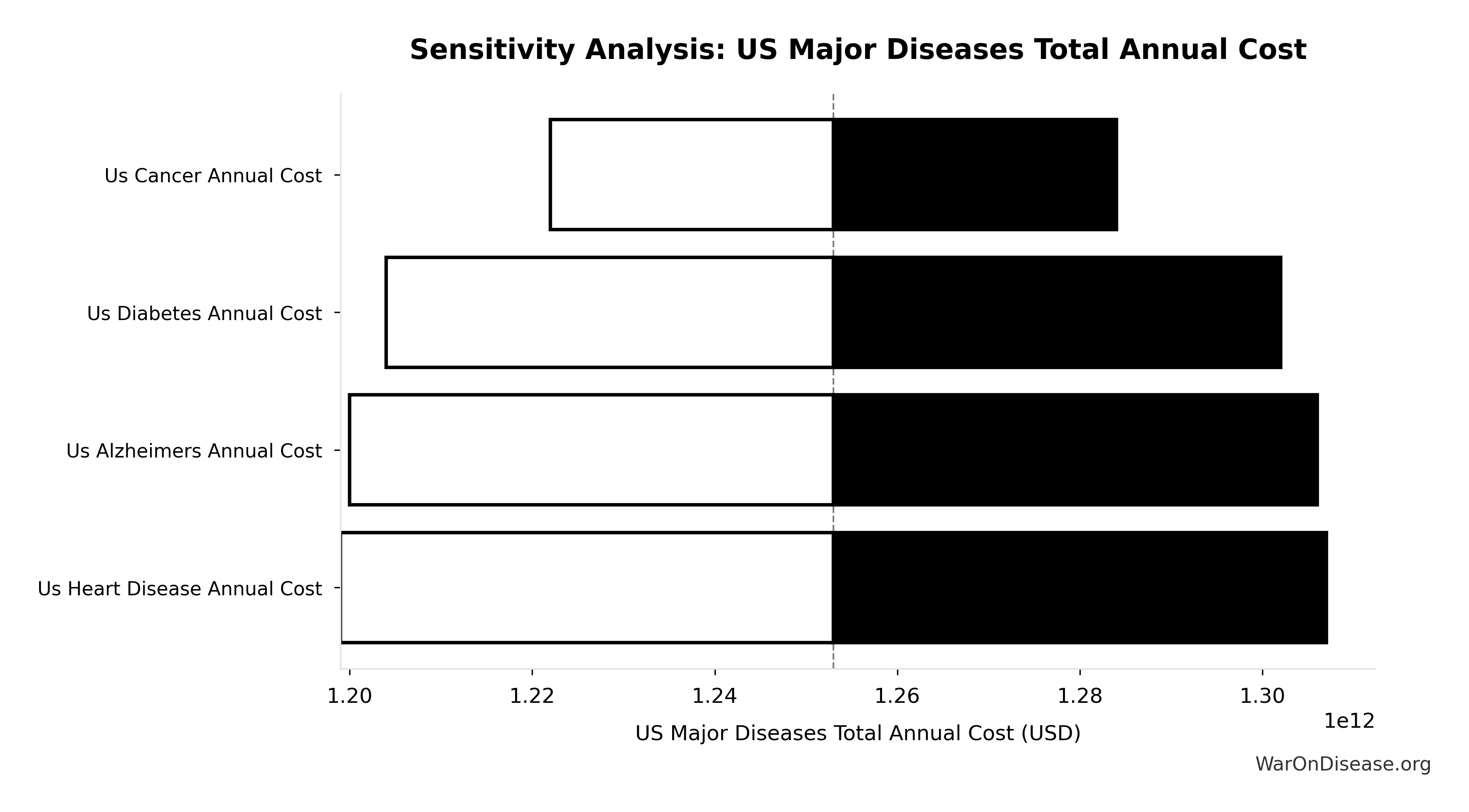
This chart shows the assumed probability distribution for this parameter. The shaded region represents the 95% confidence interval where we expect the true value to fall.
✓ High confidence
Current Trial Abandonment Rate: 40%
Note📊 Details
Annual Global Clinical Trial Participants: 1.9 million patients/year
Note📊 Details
Annual global clinical trial participants (IQVIA 2022: 1.9M post-COVID normalization)
Source:17
Uncertainty Range
Technical: 95% CI: [1.5 million patients/year, 2.3 million patients/year] • Distribution: Lognormal
What this means: This estimate has moderate uncertainty. The true value likely falls between 1.5 million patients/year and 2.3 million patients/year (±21%). This represents a reasonable range that our Monte Carlo simulations account for when calculating overall uncertainty in the results.
The lognormal distribution means values can’t go negative and have a longer tail toward higher values (common for costs and populations).
Input Distribution
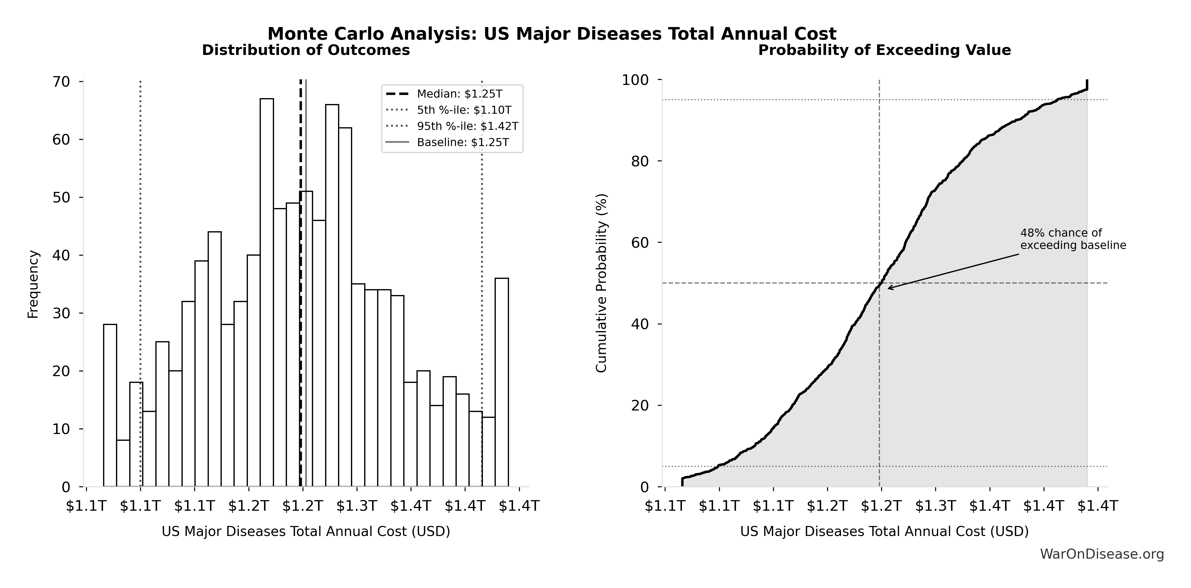
This chart shows the assumed probability distribution for this parameter. The shaded region represents the 95% confidence interval where we expect the true value to fall.
✓ High confidence
Annual Defense Industry Lobbying Spending: $127M
Note📊 Details
Annual defense industry lobbying spending
Source:19
Uncertainty Range
Technical: 95% CI: [$100M, $160M]
What this means: This estimate has moderate uncertainty. The true value likely falls between $100M and $160M (±24%). This represents a reasonable range that our Monte Carlo simulations account for when calculating overall uncertainty in the results.
Input Distribution
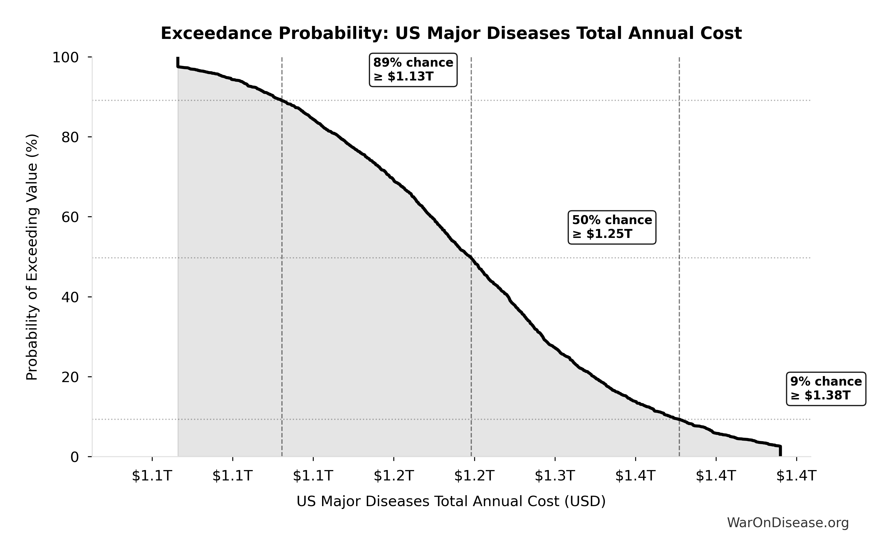
This chart shows the assumed probability distribution for this parameter. The shaded region represents the 95% confidence interval where we expect the true value to fall.
✓ High confidence • 📊 Peer-reviewed • Updated 2024
Deworming Cost per DALY: $55
Note📊 Details
Cost per DALY for deworming programs (range $28-82, midpoint estimate). GiveWell notes this 2011 estimate is outdated and their current methodology focuses on long-term income effects rather than short-term health DALYs.
Source:20
? Low confidence
dFDA Pragmatic Trial Cost per Patient: $929
Note📊 Details
dFDA pragmatic trial cost per patient. Uses ADAPTABLE trial ($929) as DELIBERATELY CONSERVATIVE central estimate. Ramsberg & Platt (2018) reviewed 108 embedded pragmatic trials; 64 with cost data had median of only $97/patient - our estimate may overstate costs by 10x. Confidence interval spans meta-analysis median to complex chronic disease trials.
Source:1
Uncertainty Range
Technical: 95% CI: [$97, $3K] • Distribution: Lognormal
What this means: This estimate is highly uncertain. The true value likely falls between $97 and $3K (±156%). This represents a very wide range that our Monte Carlo simulations account for when calculating overall uncertainty in the results.
The lognormal distribution means values can’t go negative and have a longer tail toward higher values (common for costs and populations).
Input Distribution
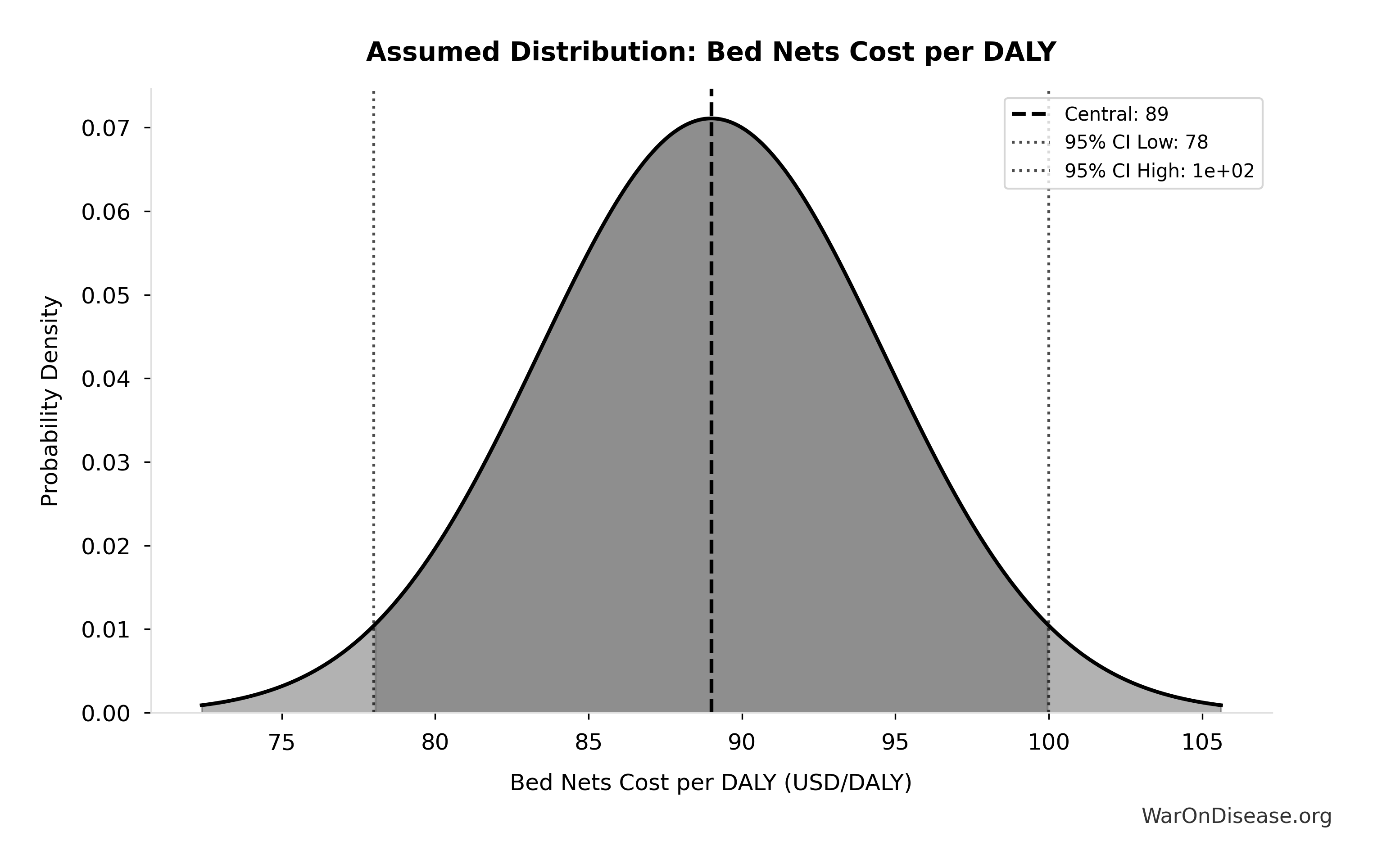
This chart shows the assumed probability distribution for this parameter. The shaded region represents the 95% confidence interval where we expect the true value to fall.
~ Medium confidence
Disease Burden as % of GDP: 13%
Note📊 Details
Fraction of GDP currently lost to disease (productivity losses + medical costs diverted from productive use). $5T productivity loss + $9.9T direct medical costs = $14.9T on $115T GDP = ~13%. As diseases are progressively cured, this drag is recovered as GDP growth. This is the missing factor that makes the treaty trajectory look like a singularity rather than a modest improvement.
Source:21
Uncertainty Range
Technical: Distribution: Fixed
✓ High confidence
Drug Development Cost (1980s): $194M
Note📊 Details
Drug development cost in 1980s (compounded to approval, 1990 dollars)
Source:23
Uncertainty Range
Technical: 95% CI: [$146M, $242M] • Distribution: Lognormal
What this means: This estimate has moderate uncertainty. The true value likely falls between $146M and $242M (±25%). This represents a reasonable range that our Monte Carlo simulations account for when calculating overall uncertainty in the results.
The lognormal distribution means values can’t go negative and have a longer tail toward higher values (common for costs and populations).
Input Distribution
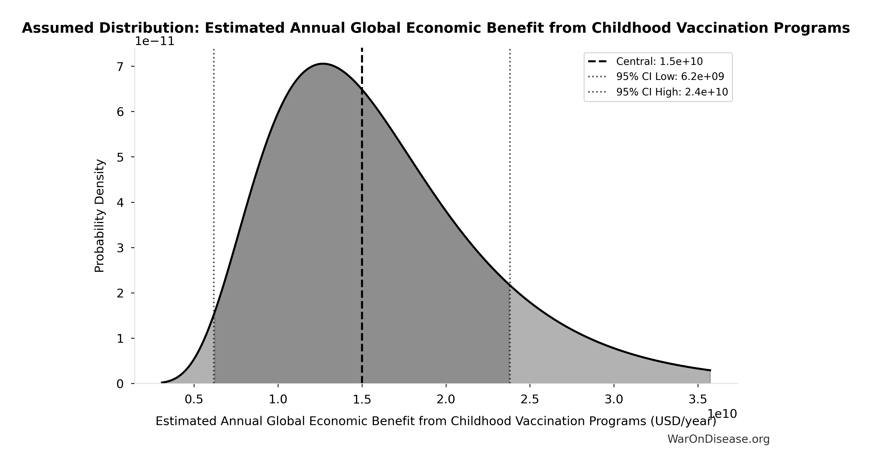
This chart shows the assumed probability distribution for this parameter. The shaded region represents the 95% confidence interval where we expect the true value to fall.
✓ High confidence
Drug Repurposing Success Rate: 30%
Note📊 Details
Percentage of drugs that gain at least one new indication after initial approval
Source:25
✓ High confidence
Economic Multiplier for Healthcare Investment: 4.3x
Note📊 Details
Economic multiplier for healthcare investment (4.3x ROI). Literature range 3.0-6.0×.
Source:27
Uncertainty Range
Technical: 95% CI: [3x, 6x] • Distribution: Lognormal
What this means: There’s significant uncertainty here. The true value likely falls between 3x and 6x (±35%). This represents a wide range that our Monte Carlo simulations account for when calculating overall uncertainty in the results.
The lognormal distribution means values can’t go negative and have a longer tail toward higher values (common for costs and populations).
Input Distribution
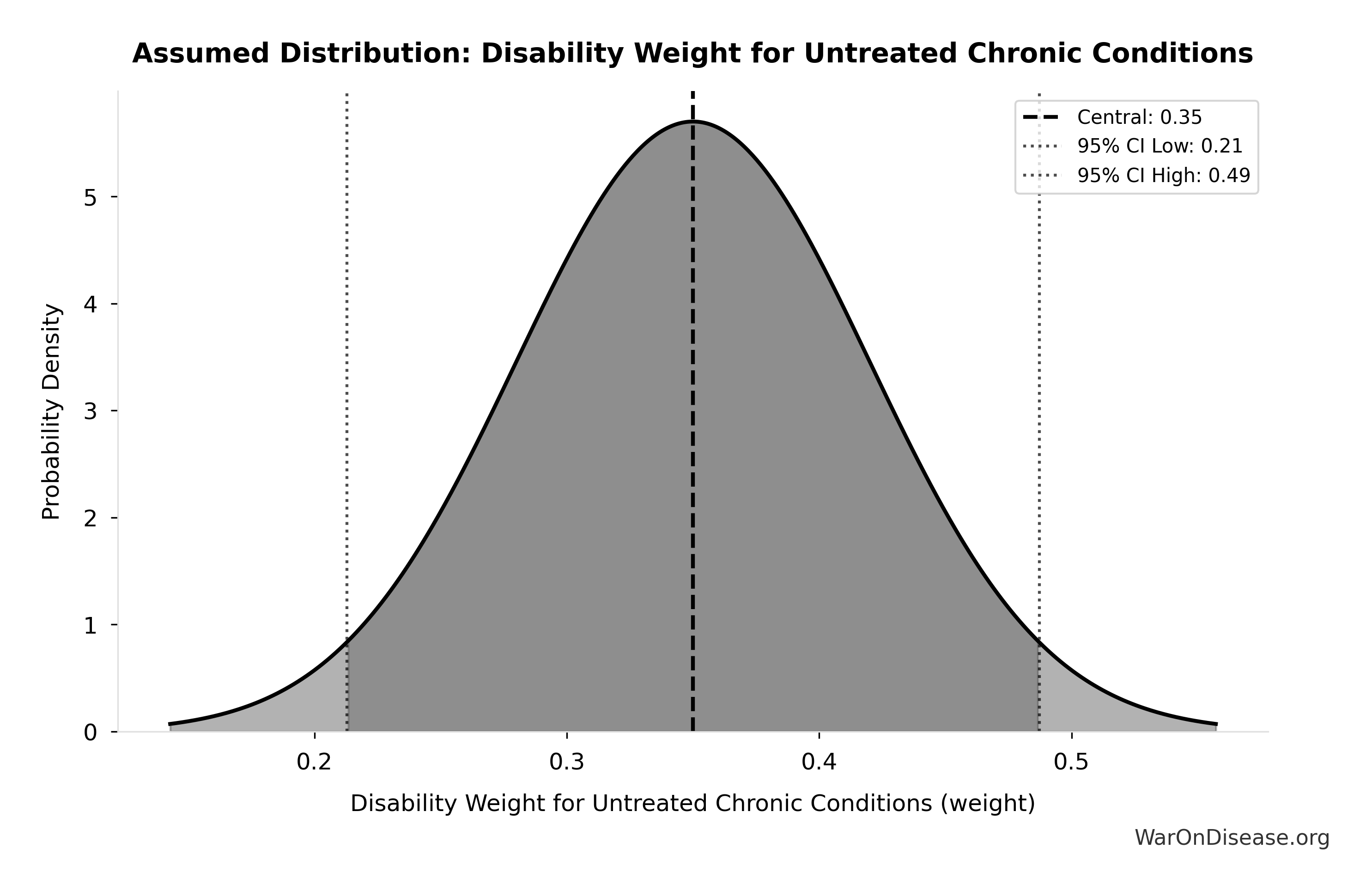
This chart shows the assumed probability distribution for this parameter. The shaded region represents the 95% confidence interval where we expect the true value to fall.
✓ High confidence
Economic Multiplier for Military Spending: 0.6x
Note📊 Details
Economic multiplier for military spending (0.6x ROI). Literature range 0.4-1.0×.
Source:29
Uncertainty Range
Technical: 95% CI: [0.4x, 0.9x] • Distribution: Lognormal
What this means: There’s significant uncertainty here. The true value likely falls between 0.4x and 0.9x (±42%). This represents a wide range that our Monte Carlo simulations account for when calculating overall uncertainty in the results.
The lognormal distribution means values can’t go negative and have a longer tail toward higher values (common for costs and populations).
Input Distribution

This chart shows the assumed probability distribution for this parameter. The shaded region represents the 95% confidence interval where we expect the true value to fall.
✓ High confidence
Regulatory Delay for Efficacy Testing Post-Safety Verification: 8.2 years
Note📊 Details
Regulatory delay for efficacy testing (Phase II/III) post-safety verification. Based on BIO 2021 industry survey. Note: This is for drugs that COMPLETE the pipeline - survivor bias means actual delay for any given disease may be longer if candidates fail and must restart.
Source:24
Uncertainty Range
Technical: Distribution: Normal (SE: 2 years)
Input Distribution
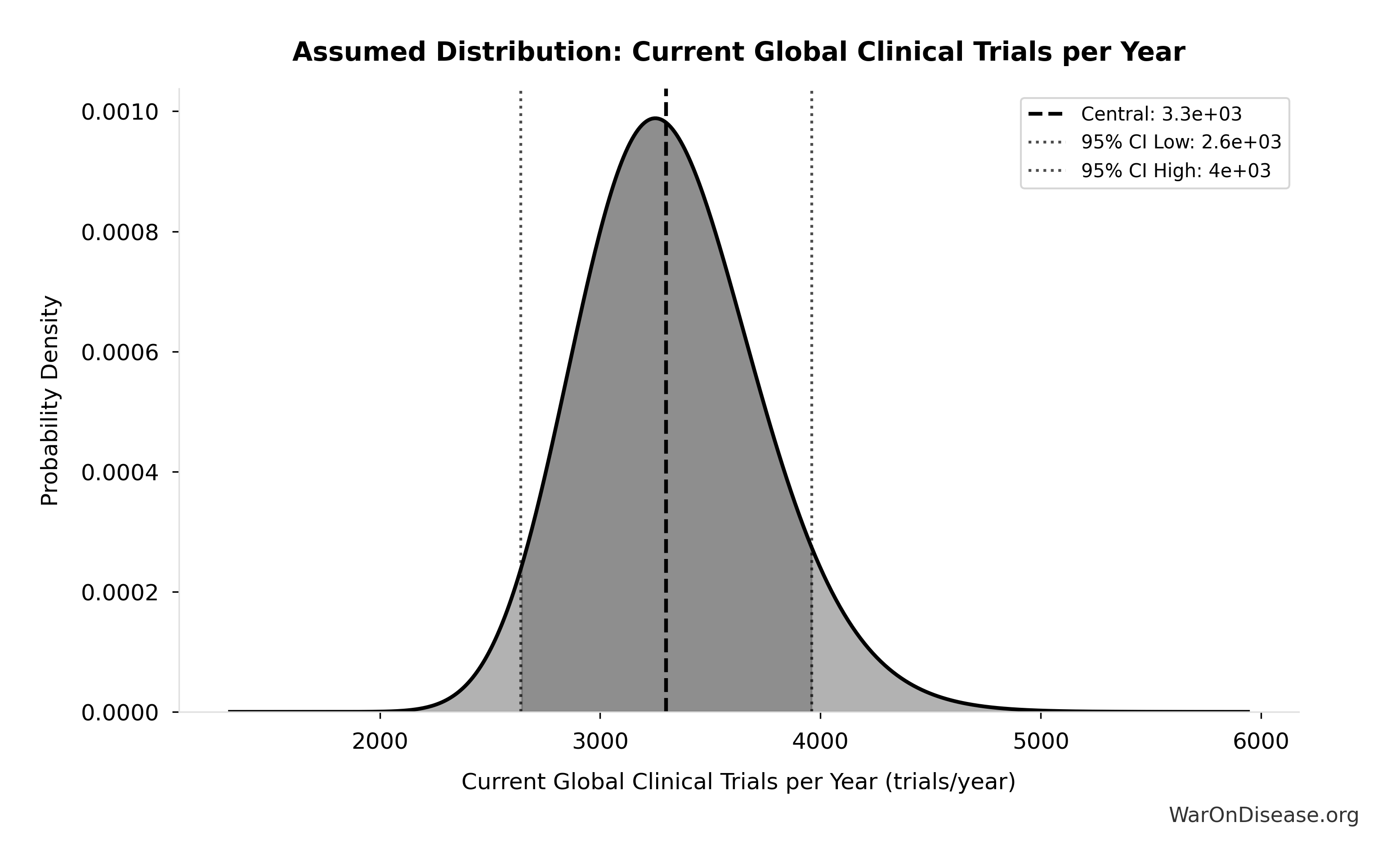
This chart shows the assumed probability distribution for this parameter. The shaded region represents the 95% confidence interval where we expect the true value to fall.
~ Medium confidence • 📊 Peer-reviewed • Updated 2021
Givewell Cost per Life Saved (Maximum): $5.5K
Note📊 Details
Givewell Cost per Life Saved (Minimum): $3.5K
Note📊 Details
Annual Deaths from Active Combat Worldwide: 234 thousand deaths/year
Note📊 Details
Annual deaths from active combat worldwide
Source:32
Uncertainty Range
Technical: 95% CI: [180 thousand deaths/year, 300 thousand deaths/year] • Distribution: Lognormal
What this means: There’s significant uncertainty here. The true value likely falls between 180 thousand deaths/year and 300 thousand deaths/year (±26%). This represents a wide range that our Monte Carlo simulations account for when calculating overall uncertainty in the results.
The lognormal distribution means values can’t go negative and have a longer tail toward higher values (common for costs and populations).
Input Distribution
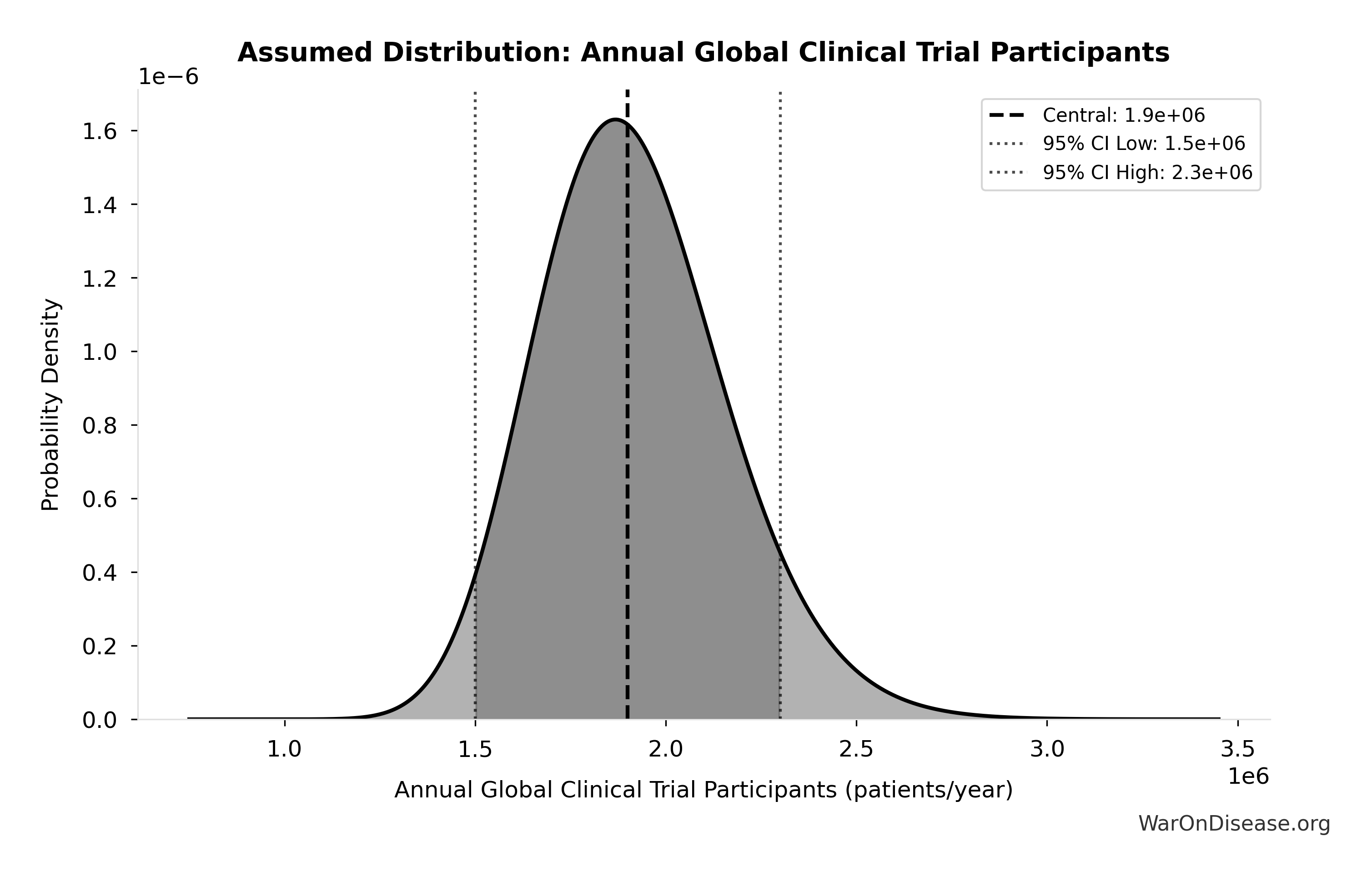
This chart shows the assumed probability distribution for this parameter. The shaded region represents the 95% confidence interval where we expect the true value to fall.
✓ High confidence
Annual Deaths from State Violence: 2.7 thousand deaths/year
Note📊 Details
Annual deaths from state violence
Source:33
Uncertainty Range
Technical: 95% CI: [1.5 thousand deaths/year, 5 thousand deaths/year] • Distribution: Lognormal
What this means: This estimate is highly uncertain. The true value likely falls between 1.5 thousand deaths/year and 5 thousand deaths/year (±65%). This represents a very wide range that our Monte Carlo simulations account for when calculating overall uncertainty in the results.
The lognormal distribution means values can’t go negative and have a longer tail toward higher values (common for costs and populations).
Input Distribution
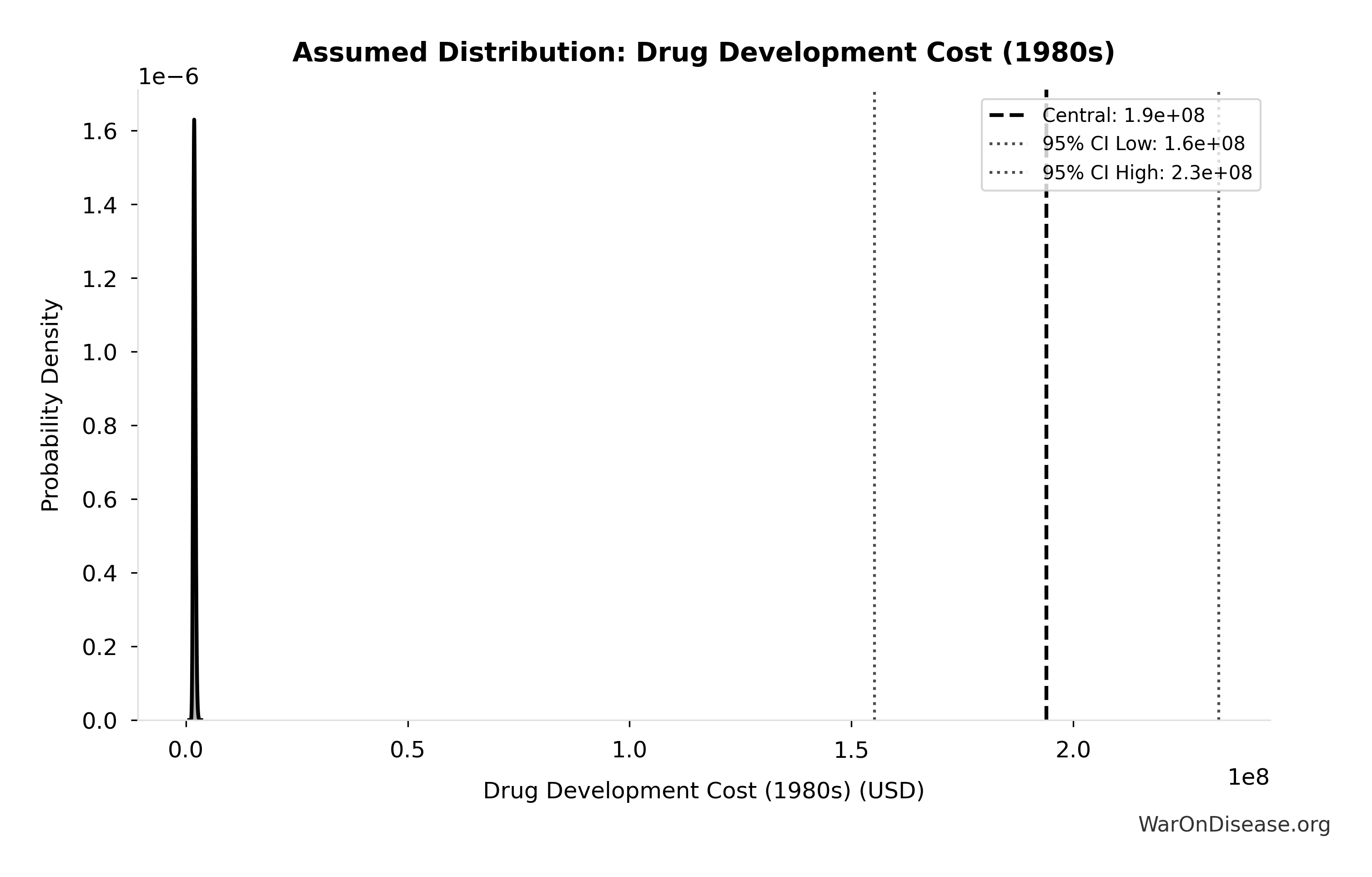
This chart shows the assumed probability distribution for this parameter. The shaded region represents the 95% confidence interval where we expect the true value to fall.
✓ High confidence
Annual Deaths from Terror Attacks Globally: 8.3 thousand deaths/year
Note📊 Details
Annual deaths from terror attacks globally
Source:34
Uncertainty Range
Technical: 95% CI: [6 thousand deaths/year, 12 thousand deaths/year] • Distribution: Lognormal
What this means: There’s significant uncertainty here. The true value likely falls between 6 thousand deaths/year and 12 thousand deaths/year (±36%). This represents a wide range that our Monte Carlo simulations account for when calculating overall uncertainty in the results.
The lognormal distribution means values can’t go negative and have a longer tail toward higher values (common for costs and populations).
Input Distribution
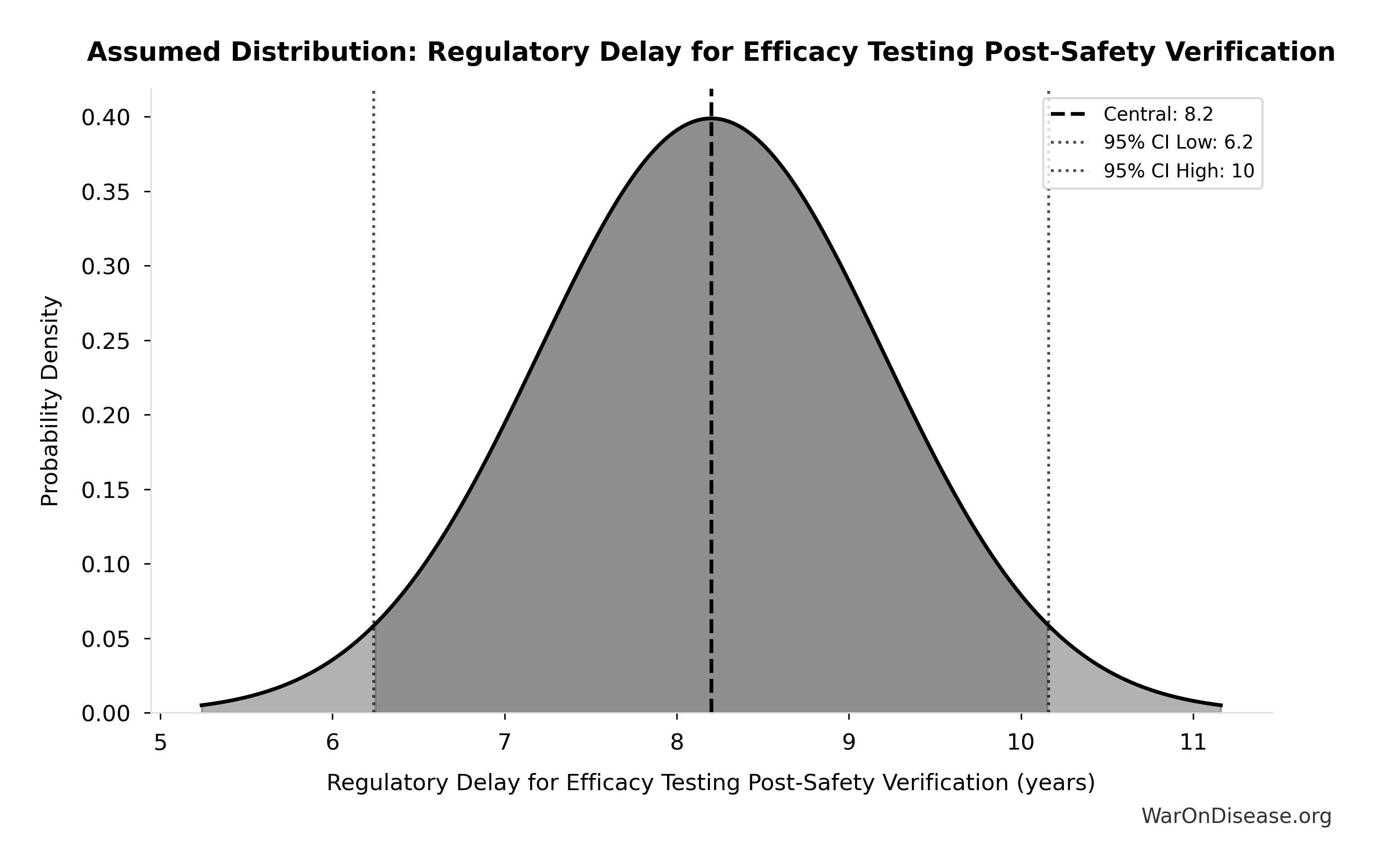
This chart shows the assumed probability distribution for this parameter. The shaded region represents the 95% confidence interval where we expect the true value to fall.
✓ High confidence
Global Annual DALY Burden: 2.88 billion DALYs/year
Note📊 Details
Global annual DALY burden from all diseases and injuries (WHO/IHME Global Burden of Disease 2021). Includes both YLL (years of life lost) and YLD (years lived with disability) from all causes.
Source:35
Uncertainty Range
Technical: Distribution: Normal (SE: 150 million DALYs/year)
Input Distribution
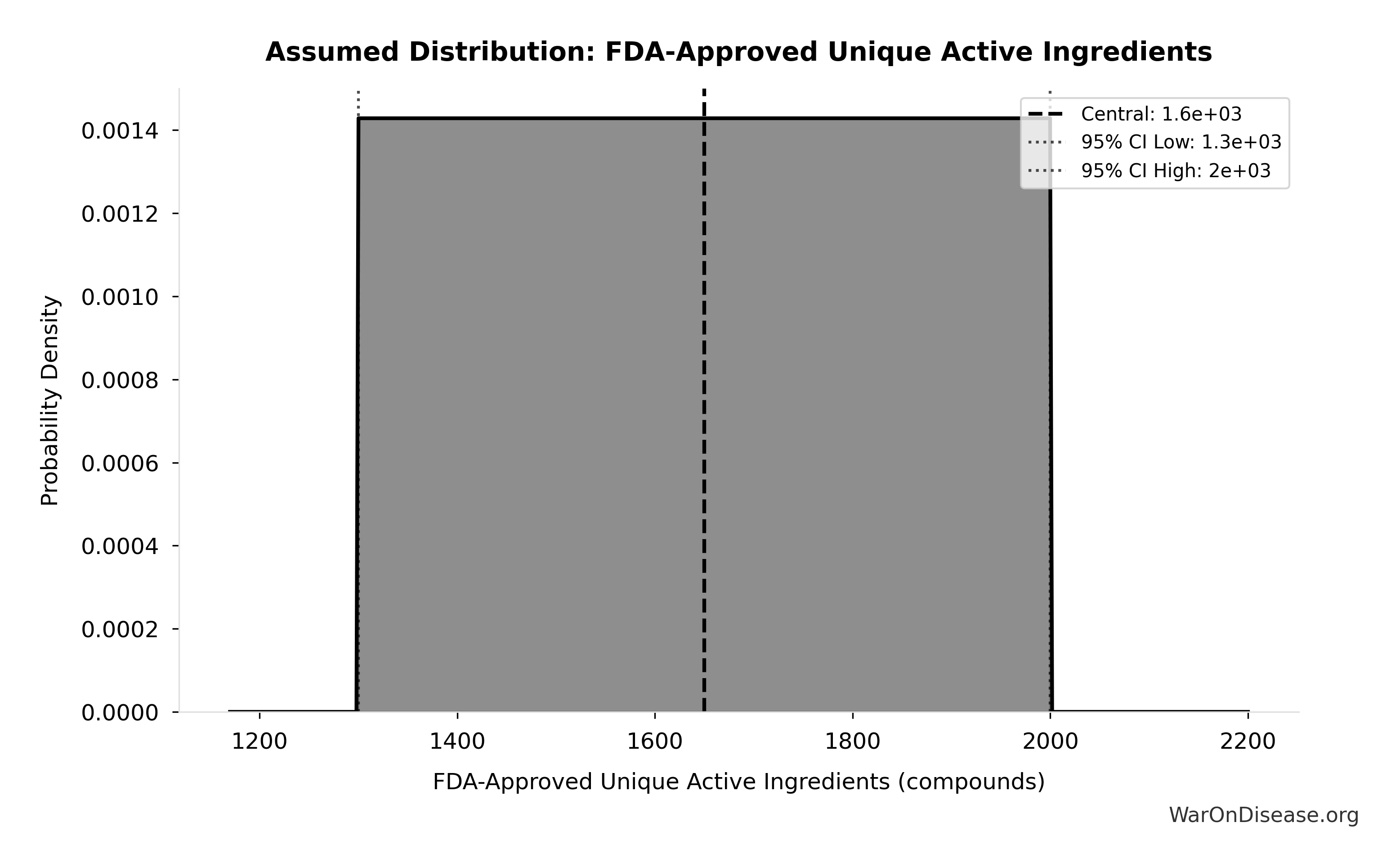
This chart shows the assumed probability distribution for this parameter. The shaded region represents the 95% confidence interval where we expect the true value to fall.
✓ High confidence • 📊 Peer-reviewed
Annual Deaths from All Diseases and Aging Globally: 55 million deaths/year
Note📊 Details
Annual deaths from all diseases and aging globally
Source:4
Uncertainty Range
Technical: Distribution: Normal (SE: 5 million deaths/year)
Input Distribution
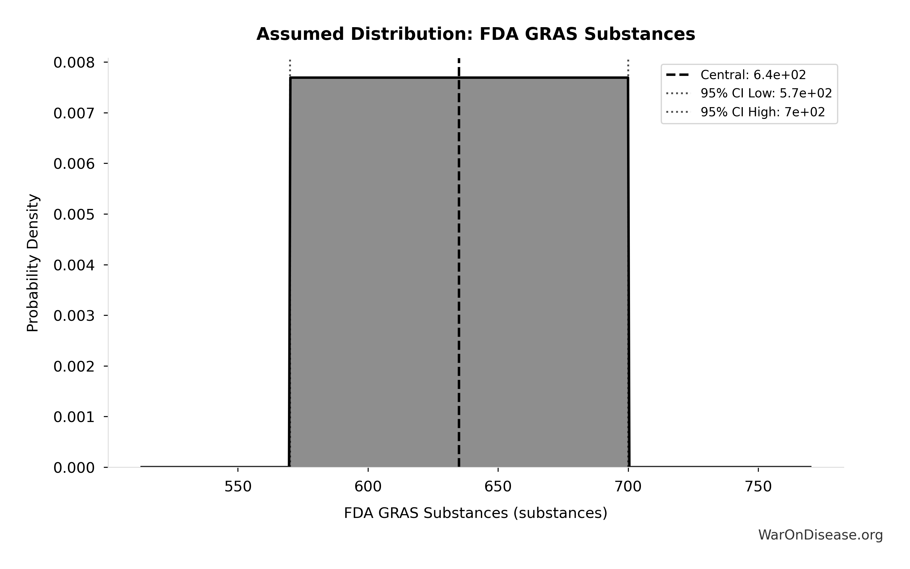
This chart shows the assumed probability distribution for this parameter. The shaded region represents the 95% confidence interval where we expect the true value to fall.
✓ High confidence
Annual Environmental Damage and Restoration Costs from Conflict: $100B
Note📊 Details
Annual environmental damage and restoration costs from conflict
Source:36
Uncertainty Range
Technical: 95% CI: [$70B, $140B] • Distribution: Lognormal
What this means: There’s significant uncertainty here. The true value likely falls between $70B and $140B (±35%). This represents a wide range that our Monte Carlo simulations account for when calculating overall uncertainty in the results.
The lognormal distribution means values can’t go negative and have a longer tail toward higher values (common for costs and populations).
Input Distribution
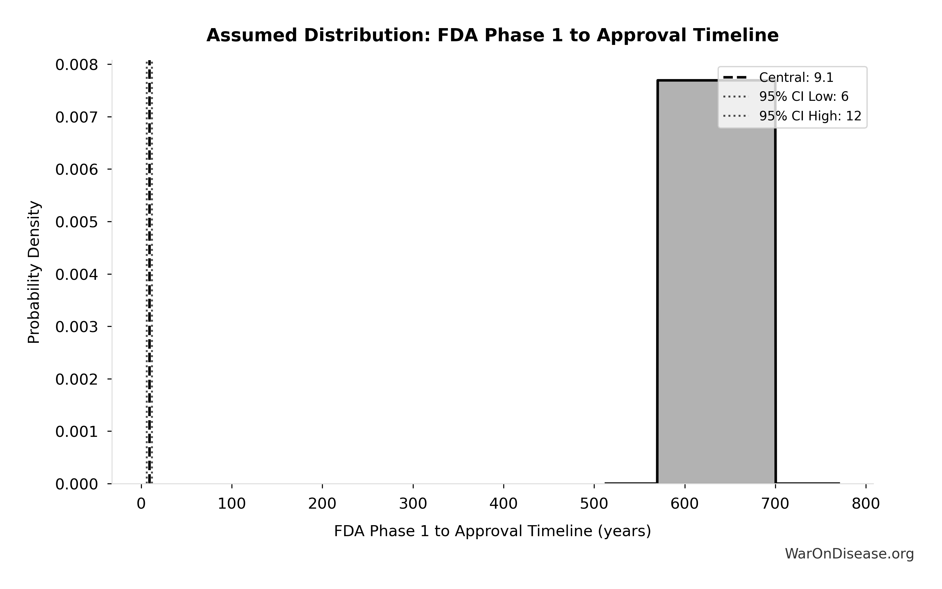
This chart shows the assumed probability distribution for this parameter. The shaded region represents the 95% confidence interval where we expect the true value to fall.
✓ High confidence
Annual Infrastructure Damage to Communications from Conflict: $298B
Note📊 Details
Annual infrastructure damage to communications from conflict
Source:36
Uncertainty Range
Technical: 95% CI: [$209B, $418B] • Distribution: Lognormal
What this means: There’s significant uncertainty here. The true value likely falls between $209B and $418B (±35%). This represents a wide range that our Monte Carlo simulations account for when calculating overall uncertainty in the results.
The lognormal distribution means values can’t go negative and have a longer tail toward higher values (common for costs and populations).
Input Distribution
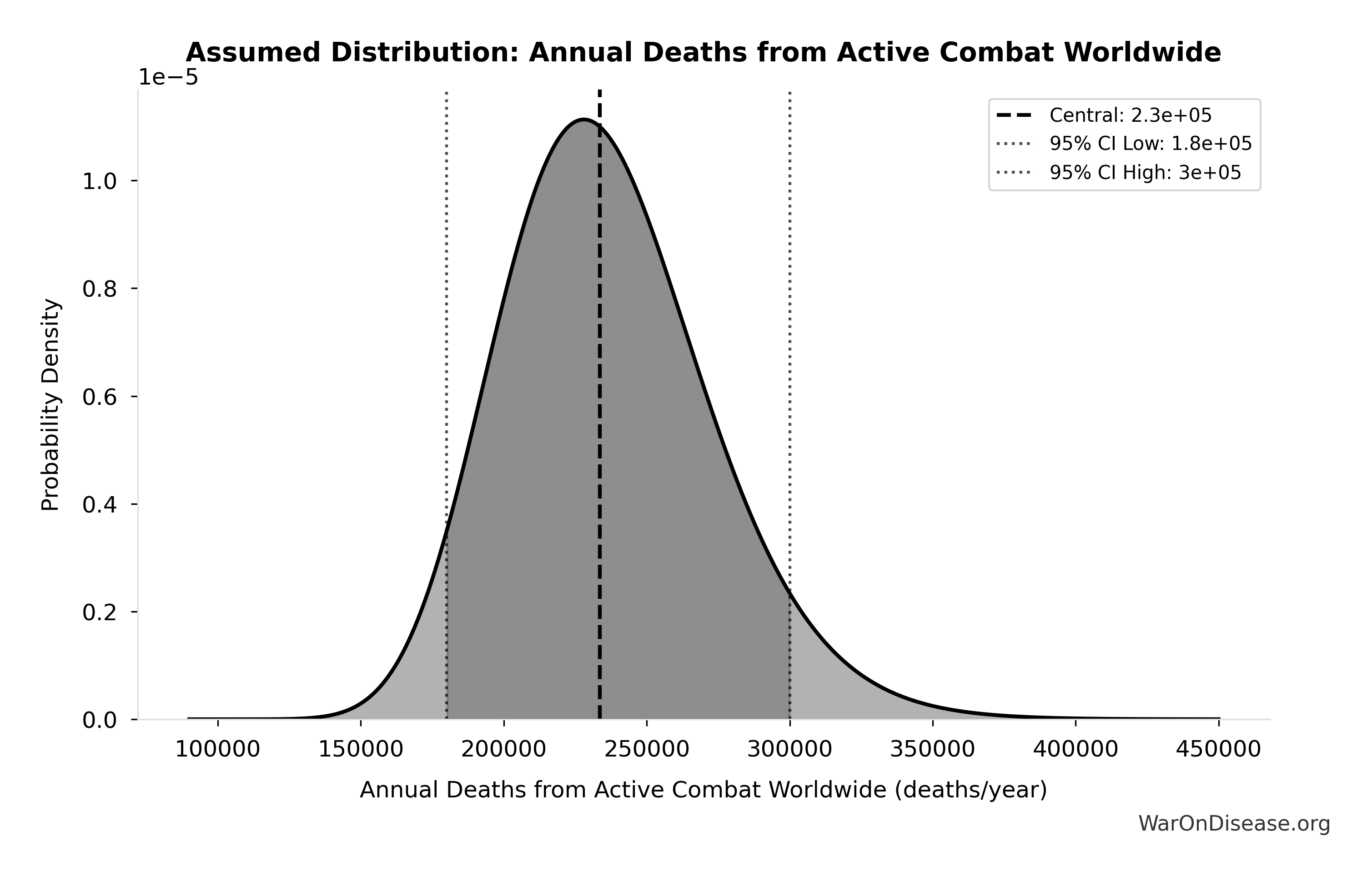
This chart shows the assumed probability distribution for this parameter. The shaded region represents the 95% confidence interval where we expect the true value to fall.
✓ High confidence
Annual Infrastructure Damage to Education Facilities from Conflict: $234B
Note📊 Details
Annual infrastructure damage to education facilities from conflict
Source:36
Uncertainty Range
Technical: 95% CI: [$164B, $328B] • Distribution: Lognormal
What this means: There’s significant uncertainty here. The true value likely falls between $164B and $328B (±35%). This represents a wide range that our Monte Carlo simulations account for when calculating overall uncertainty in the results.
The lognormal distribution means values can’t go negative and have a longer tail toward higher values (common for costs and populations).
Input Distribution
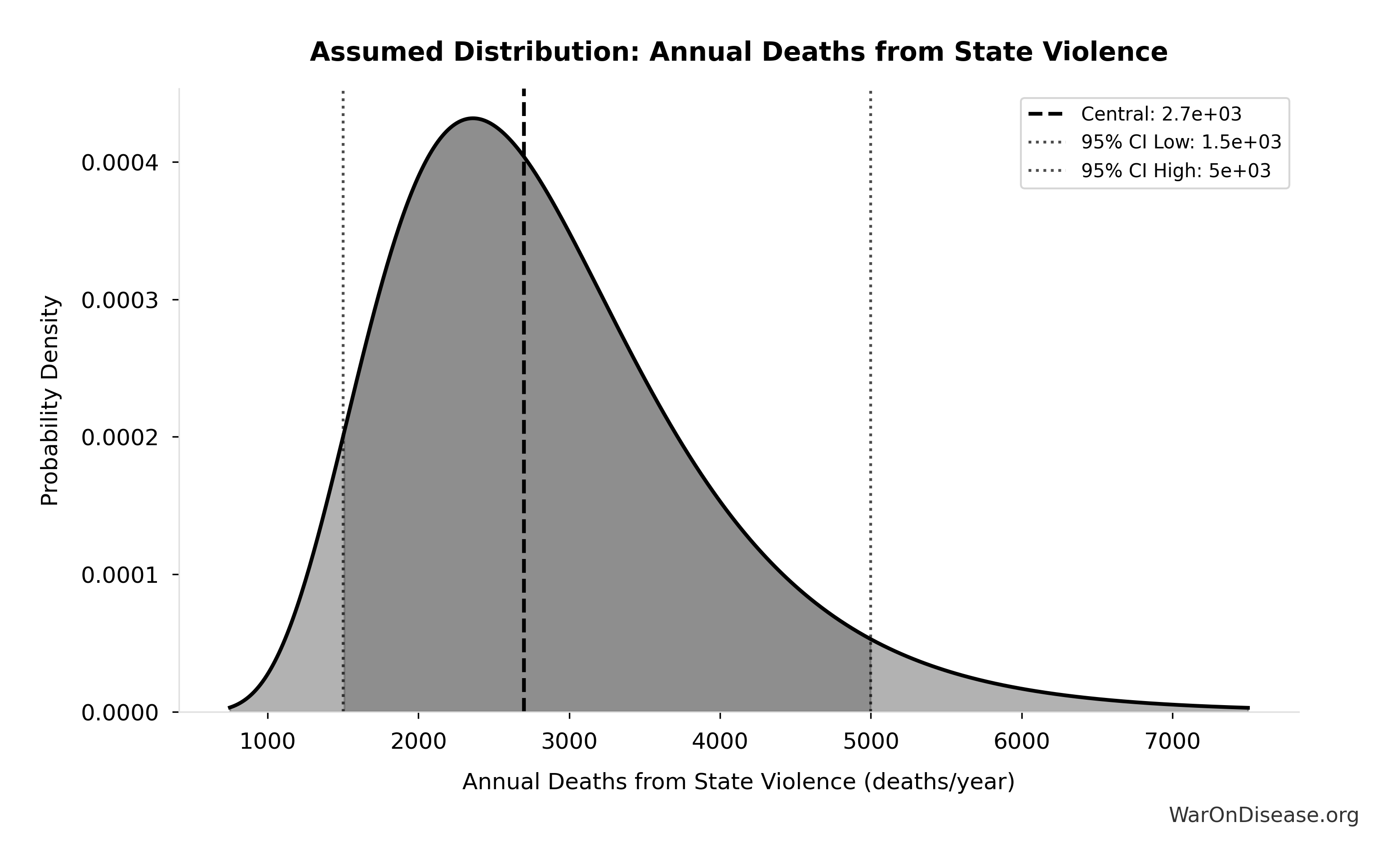
This chart shows the assumed probability distribution for this parameter. The shaded region represents the 95% confidence interval where we expect the true value to fall.
✓ High confidence
Annual Infrastructure Damage to Energy Systems from Conflict: $422B
Note📊 Details
Annual infrastructure damage to energy systems from conflict
Source:36
Uncertainty Range
Technical: 95% CI: [$295B, $590B] • Distribution: Lognormal
What this means: There’s significant uncertainty here. The true value likely falls between $295B and $590B (±35%). This represents a wide range that our Monte Carlo simulations account for when calculating overall uncertainty in the results.
The lognormal distribution means values can’t go negative and have a longer tail toward higher values (common for costs and populations).
Input Distribution
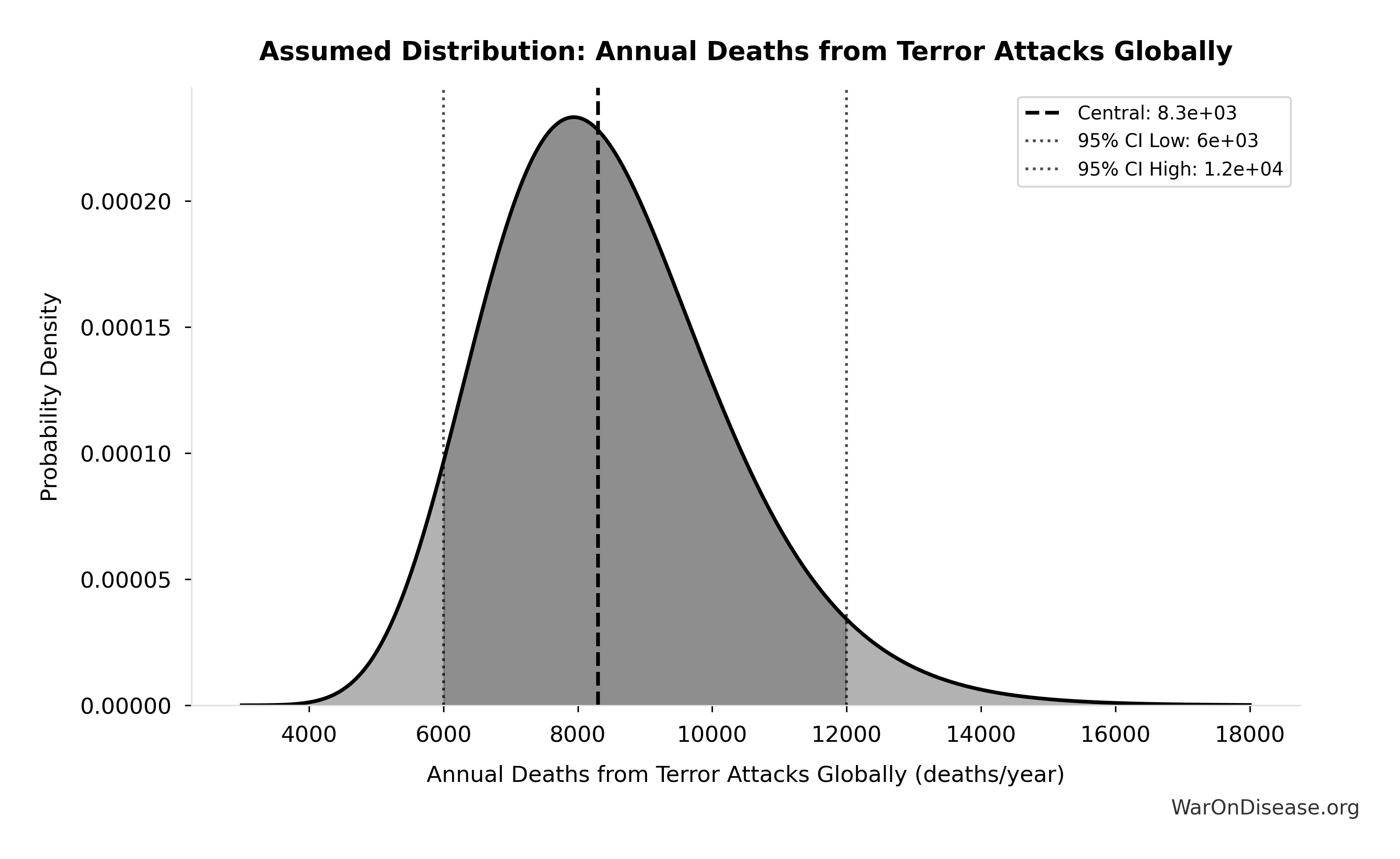
This chart shows the assumed probability distribution for this parameter. The shaded region represents the 95% confidence interval where we expect the true value to fall.
✓ High confidence
Annual Infrastructure Damage to Healthcare Facilities from Conflict: $166B
Note📊 Details
Annual infrastructure damage to healthcare facilities from conflict
Source:36
Uncertainty Range
Technical: 95% CI: [$116B, $232B] • Distribution: Lognormal
What this means: There’s significant uncertainty here. The true value likely falls between $116B and $232B (±35%). This represents a wide range that our Monte Carlo simulations account for when calculating overall uncertainty in the results.
The lognormal distribution means values can’t go negative and have a longer tail toward higher values (common for costs and populations).
Input Distribution
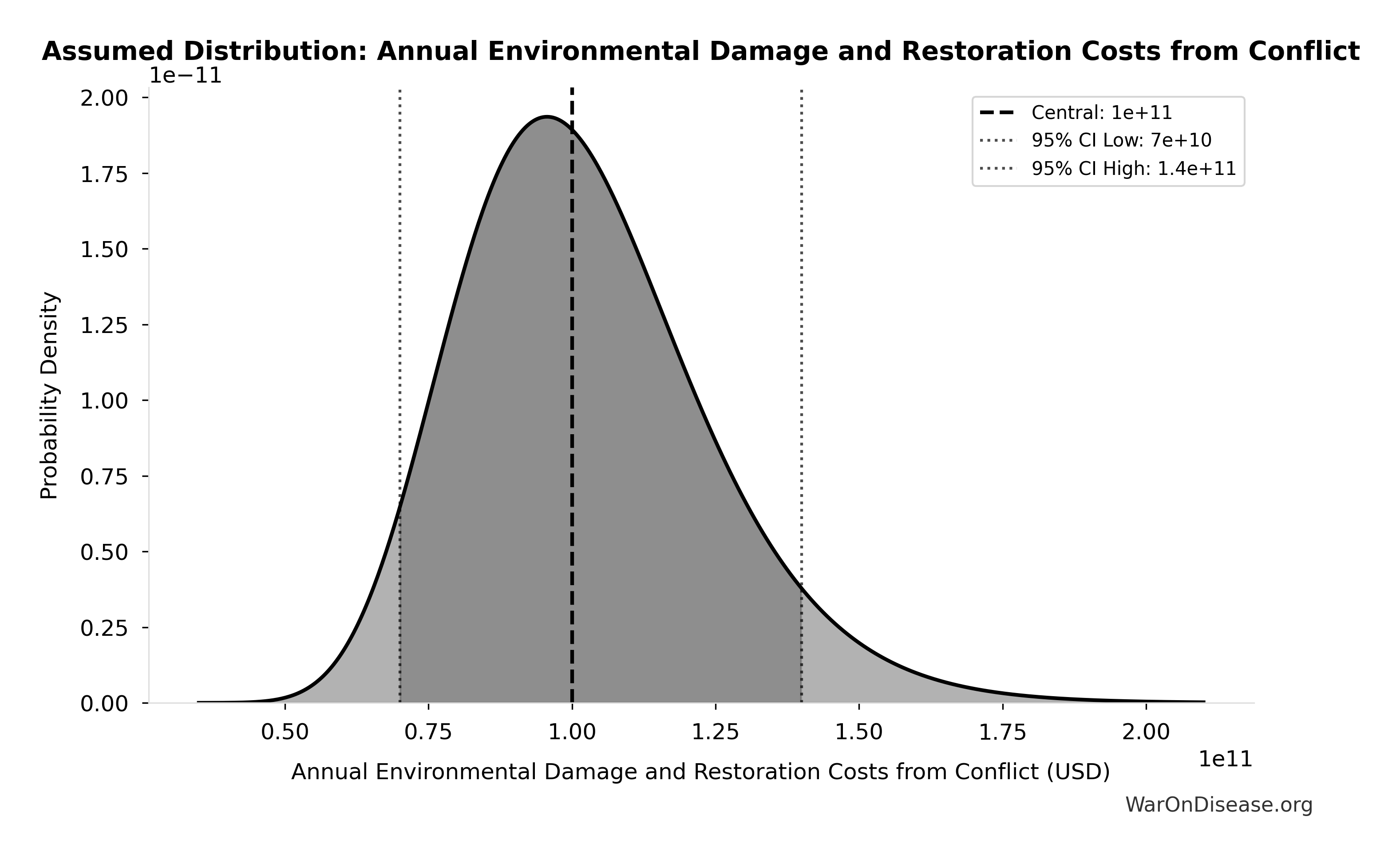
This chart shows the assumed probability distribution for this parameter. The shaded region represents the 95% confidence interval where we expect the true value to fall.
✓ High confidence
Annual Infrastructure Damage to Transportation from Conflict: $487B
Note📊 Details
Annual infrastructure damage to transportation from conflict
Source:36
Uncertainty Range
Technical: 95% CI: [$340B, $680B] • Distribution: Lognormal
What this means: There’s significant uncertainty here. The true value likely falls between $340B and $680B (±35%). This represents a wide range that our Monte Carlo simulations account for when calculating overall uncertainty in the results.
The lognormal distribution means values can’t go negative and have a longer tail toward higher values (common for costs and populations).
Input Distribution

This chart shows the assumed probability distribution for this parameter. The shaded region represents the 95% confidence interval where we expect the true value to fall.
✓ High confidence
Annual Infrastructure Damage to Water Systems from Conflict: $268B
Note📊 Details
Annual infrastructure damage to water systems from conflict
Source:36
Uncertainty Range
Technical: 95% CI: [$187B, $375B] • Distribution: Lognormal
What this means: There’s significant uncertainty here. The true value likely falls between $187B and $375B (±35%). This represents a wide range that our Monte Carlo simulations account for when calculating overall uncertainty in the results.
The lognormal distribution means values can’t go negative and have a longer tail toward higher values (common for costs and populations).
Input Distribution
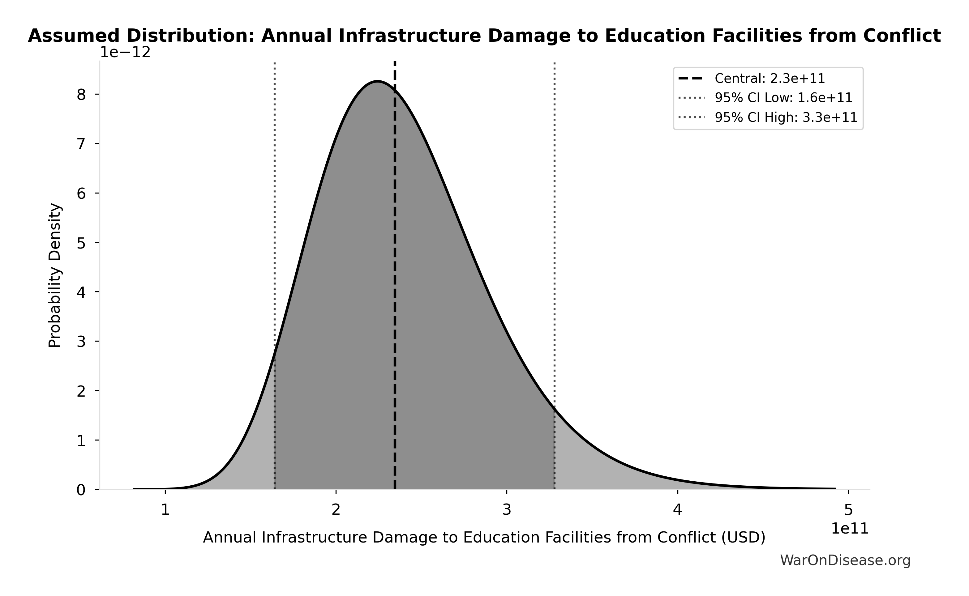
This chart shows the assumed probability distribution for this parameter. The shaded region represents the 95% confidence interval where we expect the true value to fall.
✓ High confidence
Annual Lost Economic Growth from Military Spending Opportunity Cost: $2.72T
Note📊 Details
Annual foregone economic output from military spending vs productive alternatives. This estimate implicitly captures fiscal multiplier differences (military ~0.6x vs healthcare ~4.3x GDP multiplier). Do not add separate GDP multiplier adjustment to avoid double-counting.
Source:38
Uncertainty Range
Technical: 95% CI: [$1.9T, $3.8T] • Distribution: Lognormal
What this means: There’s significant uncertainty here. The true value likely falls between $1.9T and $3.8T (±35%). This represents a wide range that our Monte Carlo simulations account for when calculating overall uncertainty in the results.
The lognormal distribution means values can’t go negative and have a longer tail toward higher values (common for costs and populations).
Input Distribution
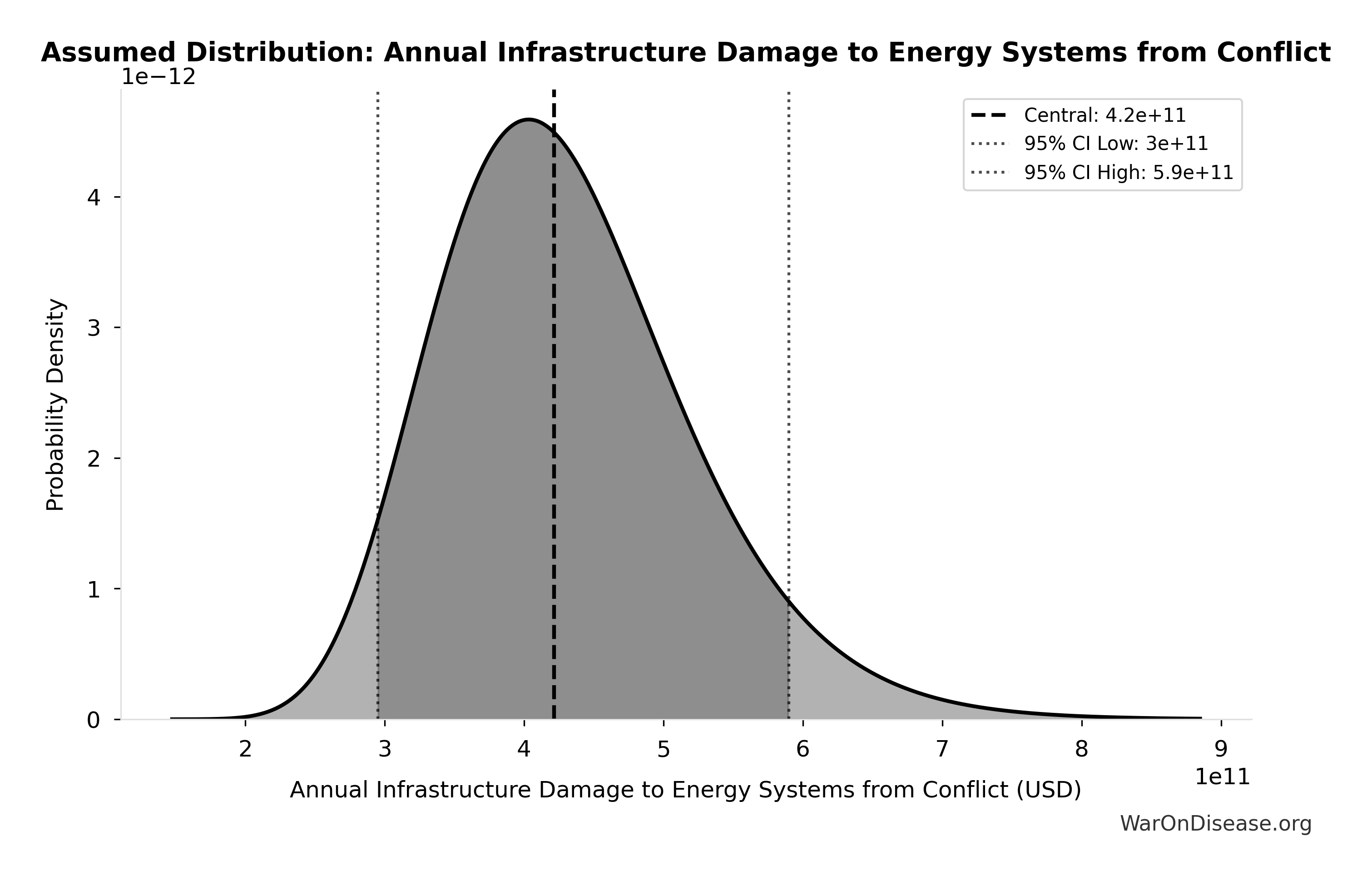
This chart shows the assumed probability distribution for this parameter. The shaded region represents the 95% confidence interval where we expect the true value to fall.
✓ High confidence
Annual Lost Productivity from Conflict Casualties: $300B
Note📊 Details
Annual lost productivity from conflict casualties
Source:39
Uncertainty Range
Technical: 95% CI: [$210B, $420B] • Distribution: Lognormal
What this means: There’s significant uncertainty here. The true value likely falls between $210B and $420B (±35%). This represents a wide range that our Monte Carlo simulations account for when calculating overall uncertainty in the results.
The lognormal distribution means values can’t go negative and have a longer tail toward higher values (common for costs and populations).
Input Distribution
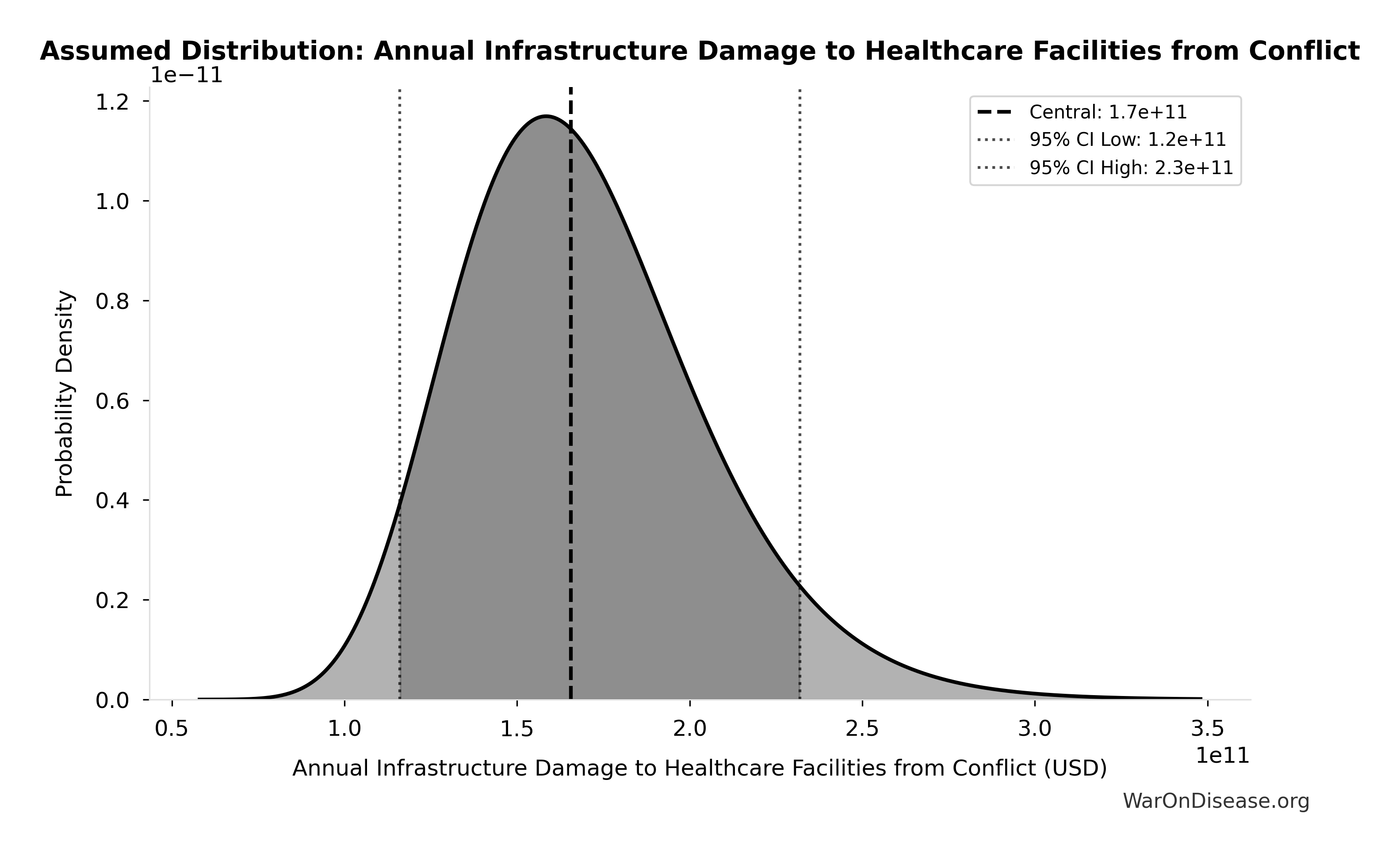
This chart shows the assumed probability distribution for this parameter. The shaded region represents the 95% confidence interval where we expect the true value to fall.
✓ High confidence
Annual PTSD and Mental Health Costs from Conflict: $232B
Note📊 Details
Annual PTSD and mental health costs from conflict
Source:40
Uncertainty Range
Technical: 95% CI: [$162B, $325B] • Distribution: Lognormal
What this means: There’s significant uncertainty here. The true value likely falls between $162B and $325B (±35%). This represents a wide range that our Monte Carlo simulations account for when calculating overall uncertainty in the results.
The lognormal distribution means values can’t go negative and have a longer tail toward higher values (common for costs and populations).
Input Distribution

This chart shows the assumed probability distribution for this parameter. The shaded region represents the 95% confidence interval where we expect the true value to fall.
✓ High confidence
Annual Refugee Support Costs: $150B
Note📊 Details
Annual refugee support costs (108.4M refugees × $1,384/year)
Source:41
Uncertainty Range
Technical: 95% CI: [$105B, $210B] • Distribution: Lognormal
What this means: There’s significant uncertainty here. The true value likely falls between $105B and $210B (±35%). This represents a wide range that our Monte Carlo simulations account for when calculating overall uncertainty in the results.
The lognormal distribution means values can’t go negative and have a longer tail toward higher values (common for costs and populations).
Input Distribution
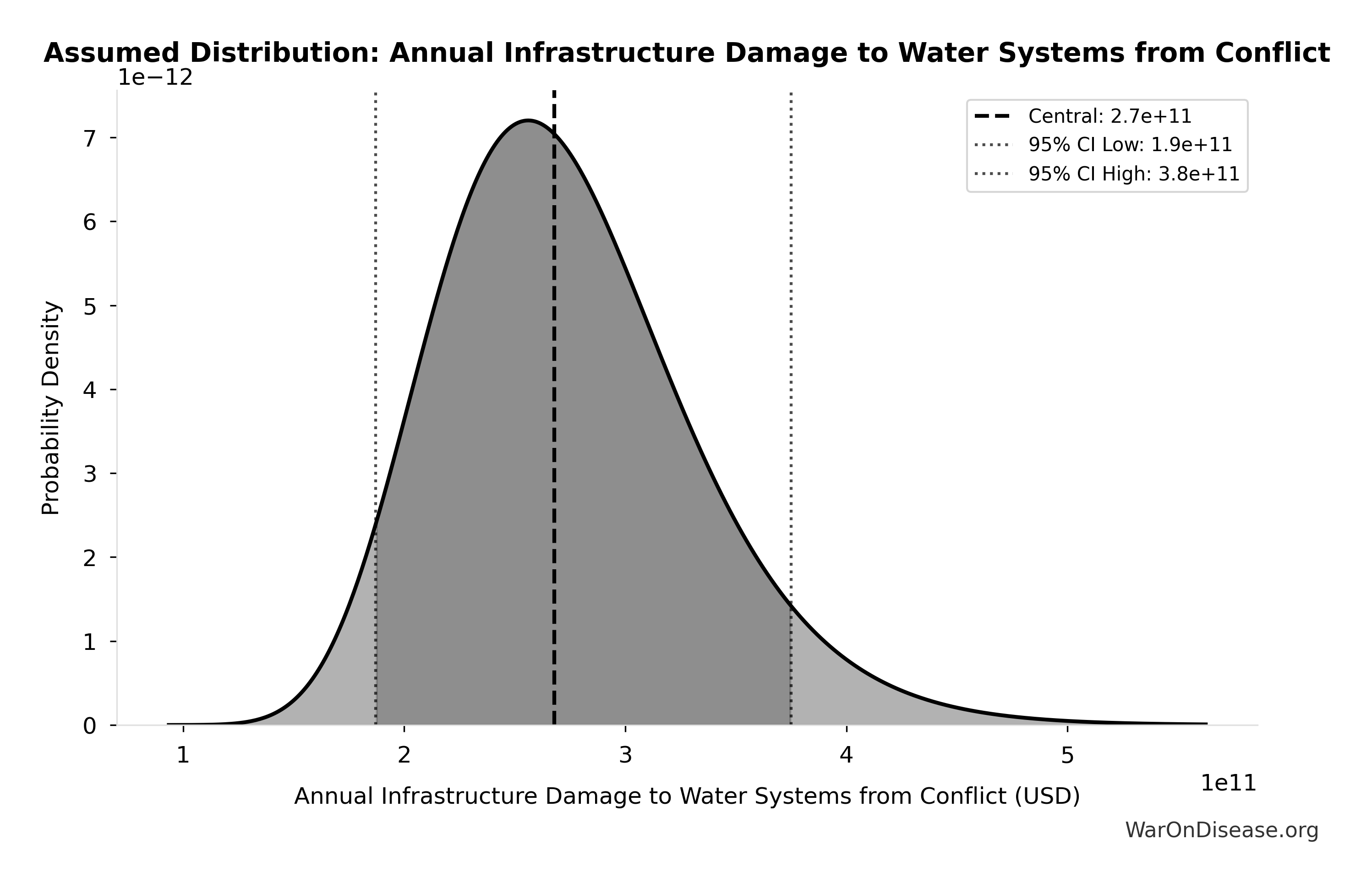
This chart shows the assumed probability distribution for this parameter. The shaded region represents the 95% confidence interval where we expect the true value to fall.
✓ High confidence
Annual Trade Disruption Costs from Currency Instability: $57.4B
Note📊 Details
Annual trade disruption costs from currency instability
Source:42
Uncertainty Range
Technical: 95% CI: [$40B, $80B] • Distribution: Lognormal
What this means: There’s significant uncertainty here. The true value likely falls between $40B and $80B (±35%). This represents a wide range that our Monte Carlo simulations account for when calculating overall uncertainty in the results.
The lognormal distribution means values can’t go negative and have a longer tail toward higher values (common for costs and populations).
Input Distribution
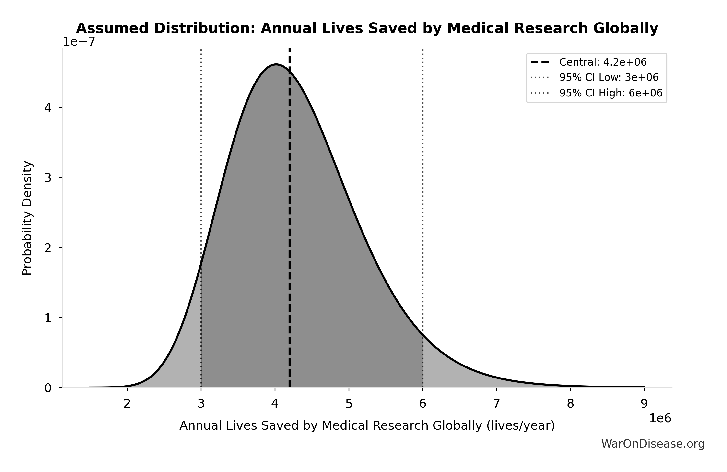
This chart shows the assumed probability distribution for this parameter. The shaded region represents the 95% confidence interval where we expect the true value to fall.
✓ High confidence
Annual Trade Disruption Costs from Energy Price Volatility: $125B
Note📊 Details
Annual trade disruption costs from energy price volatility
Source:42
Uncertainty Range
Technical: 95% CI: [$87B, $175B] • Distribution: Lognormal
What this means: There’s significant uncertainty here. The true value likely falls between $87B and $175B (±35%). This represents a wide range that our Monte Carlo simulations account for when calculating overall uncertainty in the results.
The lognormal distribution means values can’t go negative and have a longer tail toward higher values (common for costs and populations).
Input Distribution

This chart shows the assumed probability distribution for this parameter. The shaded region represents the 95% confidence interval where we expect the true value to fall.
✓ High confidence
Annual Trade Disruption Costs from Shipping Disruptions: $247B
Note📊 Details
Annual trade disruption costs from shipping disruptions
Source:42
Uncertainty Range
Technical: 95% CI: [$173B, $346B] • Distribution: Lognormal
What this means: There’s significant uncertainty here. The true value likely falls between $173B and $346B (±35%). This represents a wide range that our Monte Carlo simulations account for when calculating overall uncertainty in the results.
The lognormal distribution means values can’t go negative and have a longer tail toward higher values (common for costs and populations).
Input Distribution

This chart shows the assumed probability distribution for this parameter. The shaded region represents the 95% confidence interval where we expect the true value to fall.
✓ High confidence
Annual Trade Disruption Costs from Supply Chain Disruptions: $187B
Note📊 Details
Annual trade disruption costs from supply chain disruptions
Source:42
Uncertainty Range
Technical: 95% CI: [$131B, $262B] • Distribution: Lognormal
What this means: There’s significant uncertainty here. The true value likely falls between $131B and $262B (±35%). This represents a wide range that our Monte Carlo simulations account for when calculating overall uncertainty in the results.
The lognormal distribution means values can’t go negative and have a longer tail toward higher values (common for costs and populations).
Input Distribution

This chart shows the assumed probability distribution for this parameter. The shaded region represents the 95% confidence interval where we expect the true value to fall.
✓ High confidence
Annual Veteran Healthcare Costs: $200B
Note📊 Details
Annual veteran healthcare costs (20-year projected)
Source:43
Uncertainty Range
Technical: 95% CI: [$140B, $280B] • Distribution: Lognormal
What this means: There’s significant uncertainty here. The true value likely falls between $140B and $280B (±35%). This represents a wide range that our Monte Carlo simulations account for when calculating overall uncertainty in the results.
The lognormal distribution means values can’t go negative and have a longer tail toward higher values (common for costs and populations).
Input Distribution
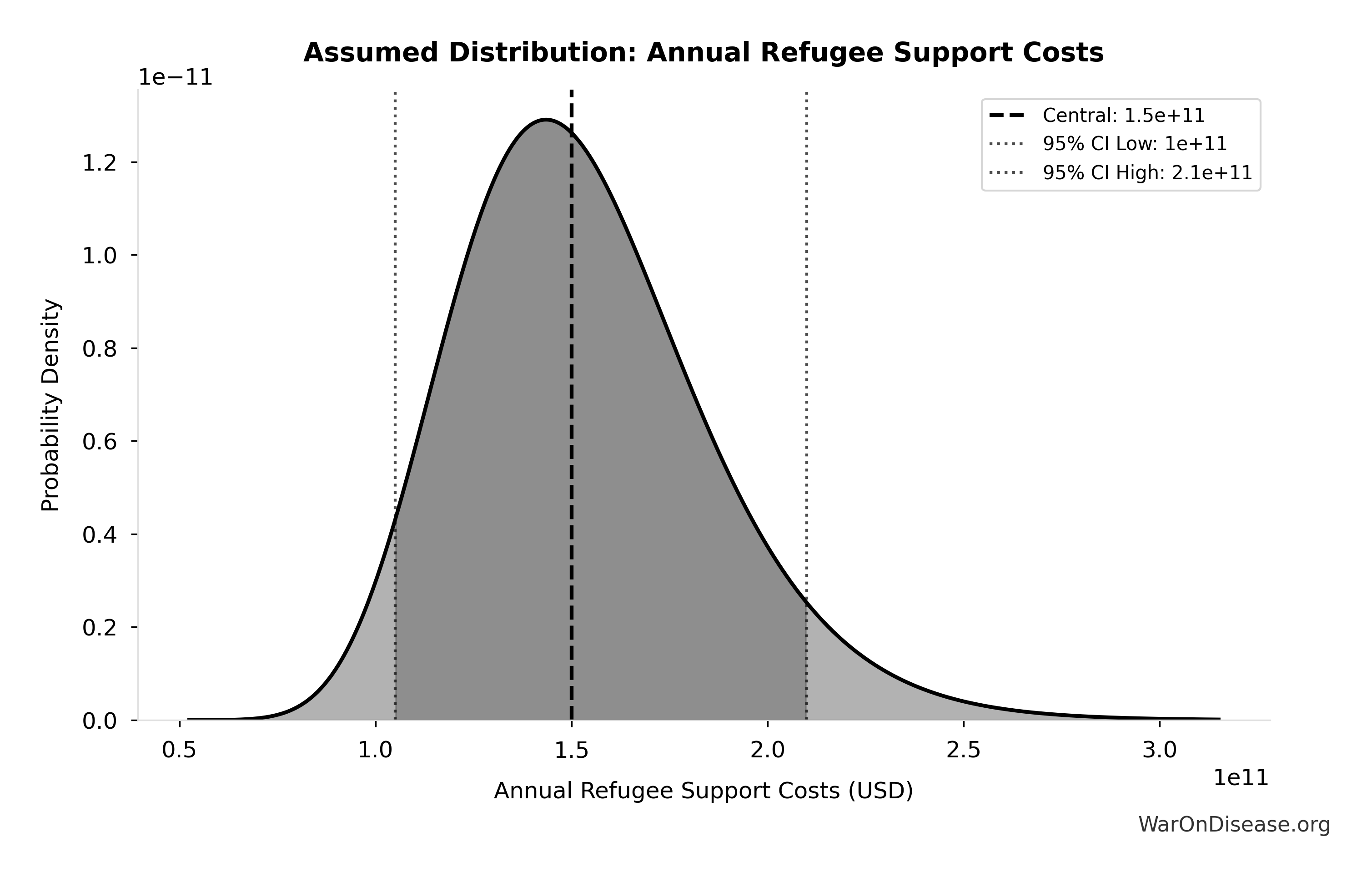
This chart shows the assumed probability distribution for this parameter. The shaded region represents the 95% confidence interval where we expect the true value to fall.
✓ High confidence
Annual Global Spending on Clinical Trials: $60B
Note📊 Details
Annual global spending on clinical trials (Industry: $45-60B + Government: $3-6B + Nonprofits: $2-5B). Conservative estimate using 15-20% of $300B total pharma R&D, not inflated market size projections.
Source:45
Uncertainty Range
Technical: 95% CI: [$50B, $75B] • Distribution: Lognormal (SE: $10B)
What this means: This estimate has moderate uncertainty. The true value likely falls between $50B and $75B (±21%). This represents a reasonable range that our Monte Carlo simulations account for when calculating overall uncertainty in the results.
The lognormal distribution means values can’t go negative and have a longer tail toward higher values (common for costs and populations).
Input Distribution
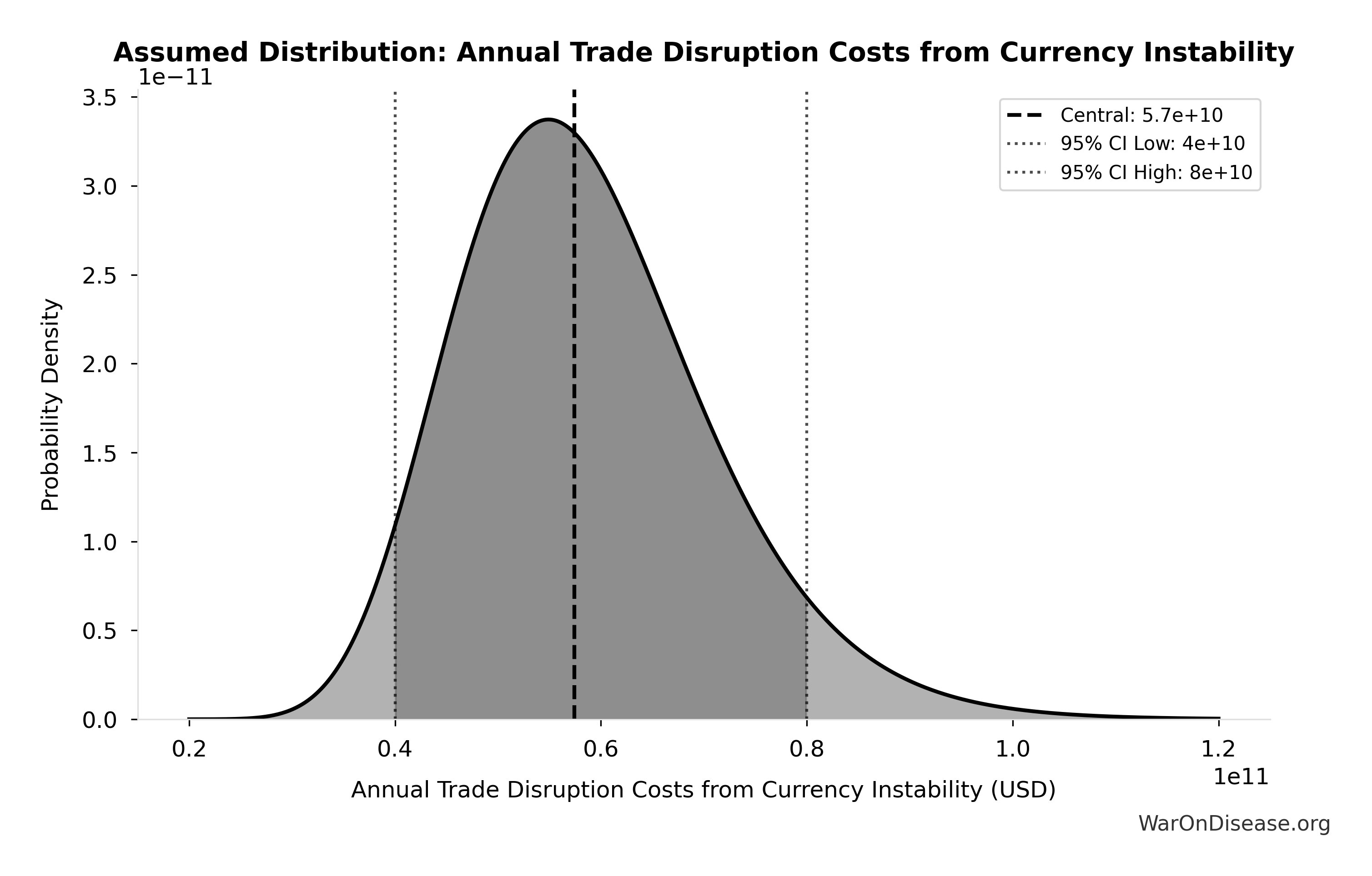
This chart shows the assumed probability distribution for this parameter. The shaded region represents the 95% confidence interval where we expect the true value to fall.
✓ High confidence
Global Daily Deaths from Disease and Aging: 150 thousand deaths/day
Note📊 Details
Total global deaths per day from all disease and aging (WHO Global Burden of Disease 2024)
Source:4
Uncertainty Range
Technical: Distribution: Normal (SE: 7.5 thousand deaths/day)
Input Distribution

This chart shows the assumed probability distribution for this parameter. The shaded region represents the 95% confidence interval where we expect the true value to fall.
✓ High confidence • 📊 Peer-reviewed
Global GDP (2025): $115T
Note📊 Details
Global nominal GDP (2025 estimate). From Political Dysfunction Tax paper citing StatisticsTimes/IMF World Economic Outlook. Used for calculating global opportunity costs as percentage of world economic output. Note: Latest IMF data shows $117T.
Source:47
Uncertainty Range
Technical: Distribution: Fixed
✓ High confidence
Annual Global Government Spending on Clinical Trials: $4.5B
Note📊 Details
Annual global government spending on interventional clinical trials (~5-10% of total)
Source:48
Uncertainty Range
Technical: 95% CI: [$3B, $6B] • Distribution: Lognormal (SE: $1B)
What this means: There’s significant uncertainty here. The true value likely falls between $3B and $6B (±33%). This represents a wide range that our Monte Carlo simulations account for when calculating overall uncertainty in the results.
The lognormal distribution means values can’t go negative and have a longer tail toward higher values (common for costs and populations).
Input Distribution
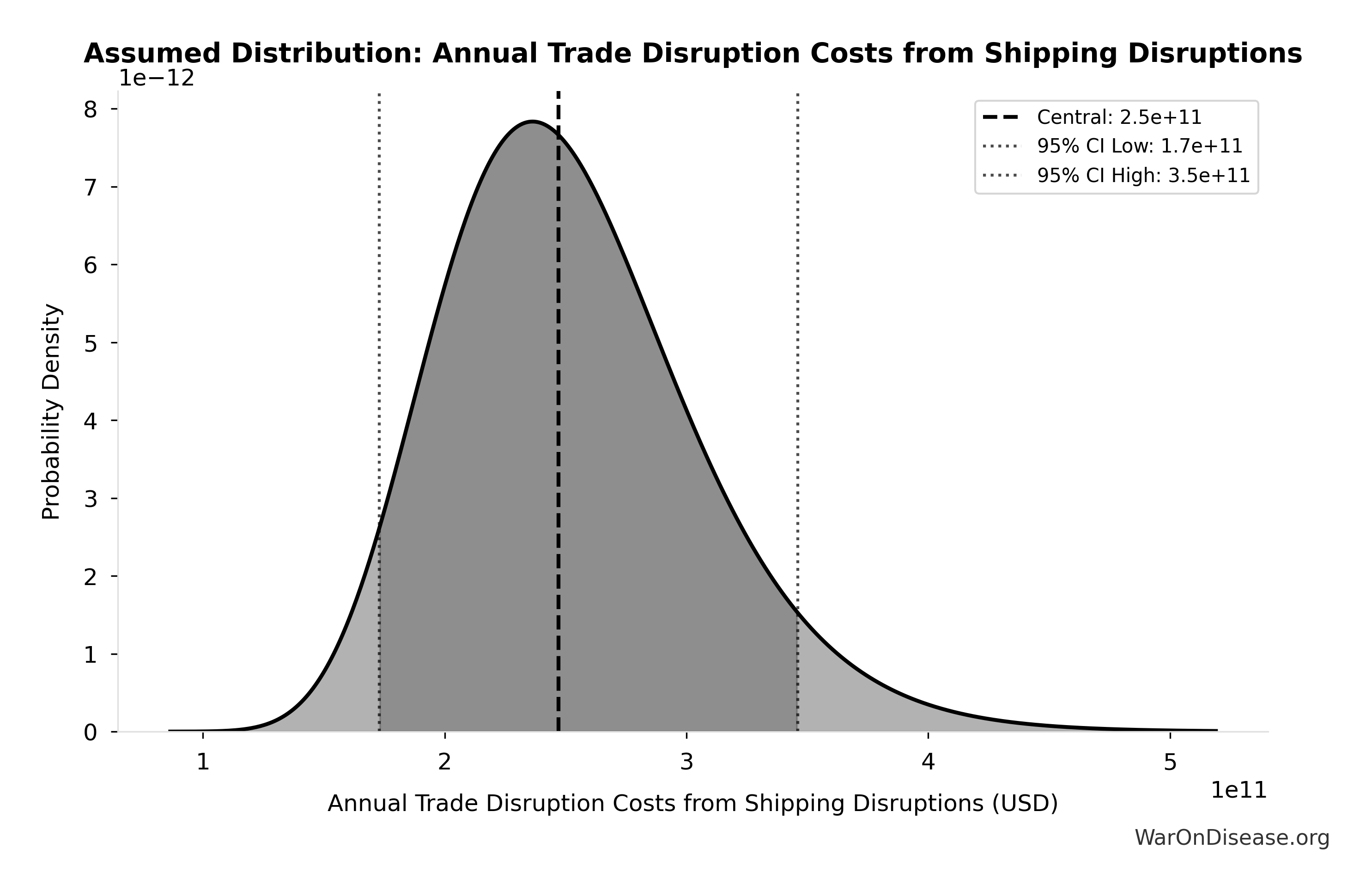
This chart shows the assumed probability distribution for this parameter. The shaded region represents the 95% confidence interval where we expect the true value to fall.
✓ High confidence
Global Life Expectancy (2024): 79 years
Note📊 Details
Global life expectancy (2024)
Source:4
Uncertainty Range
Technical: Distribution: Normal (SE: 2 years)
Input Distribution

This chart shows the assumed probability distribution for this parameter. The shaded region represents the 95% confidence interval where we expect the true value to fall.
✓ High confidence • 📊 Peer-reviewed • Updated 2024
Global Government Medical Research Spending: $67.5B
Note📊 Details
Global government medical research spending
Source:50
Uncertainty Range
Technical: 95% CI: [$54B, $81B] • Distribution: Lognormal
What this means: This estimate has moderate uncertainty. The true value likely falls between $54B and $81B (±20%). This represents a reasonable range that our Monte Carlo simulations account for when calculating overall uncertainty in the results.
The lognormal distribution means values can’t go negative and have a longer tail toward higher values (common for costs and populations).
Input Distribution

This chart shows the assumed probability distribution for this parameter. The shaded region represents the 95% confidence interval where we expect the true value to fall.
✓ High confidence
Global Military Spending in 2024: $2.72T
Note📊 Details
Global military spending in 2024
Source:52
Uncertainty Range
Technical: Distribution: Fixed
✓ High confidence
Global Population in 2024: 8 billion of people
Note📊 Details
Global population in 2024
Source:56
Uncertainty Range
Technical: 95% CI: [7.8 billion of people, 8.2 billion of people] • Distribution: Lognormal
What this means: We’re quite confident in this estimate. The true value likely falls between 7.8 billion of people and 8.2 billion of people (±2%). This represents a narrow range that our Monte Carlo simulations account for when calculating overall uncertainty in the results.
The lognormal distribution means values can’t go negative and have a longer tail toward higher values (common for costs and populations).
Input Distribution

This chart shows the assumed probability distribution for this parameter. The shaded region represents the 95% confidence interval where we expect the true value to fall.
✓ High confidence
Global Population 2045 (Projected): 9.2 billion of people
Note📊 Details
UN World Population Prospects 2022 median projection for 2045.
Source:56
Uncertainty Range
Technical: Distribution: Fixed
✓ High confidence
Critical Mass Threshold for Social Change: 3.5%
Note📊 Details
Critical mass threshold for social change (3.5% rule). Chenoweth studied national regime changes; applying to a global treaty adds uncertainty. Lower bound: some movements succeeded at ~1%. Upper bound: entrenched defense-industry opposition and weaker signal from digital signatures vs sustained protest may require up to 10%.
Source:57
Uncertainty Range
Technical: 95% CI: [1%, 10%] • Distribution: Lognormal
What this means: This estimate is highly uncertain. The true value likely falls between 1% and 10% (±129%). This represents a very wide range that our Monte Carlo simulations account for when calculating overall uncertainty in the results.
The lognormal distribution means values can’t go negative and have a longer tail toward higher values (common for costs and populations).
Input Distribution
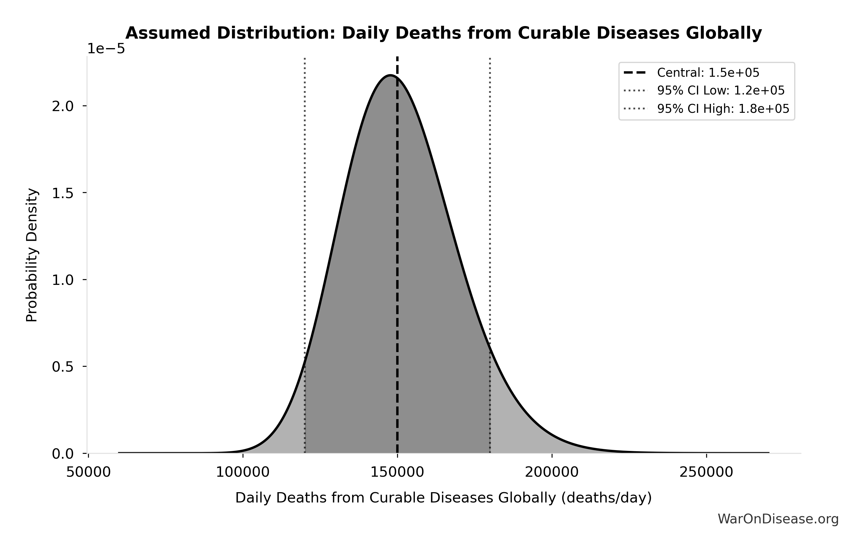
This chart shows the assumed probability distribution for this parameter. The shaded region represents the 95% confidence interval where we expect the true value to fall.
✓ High confidence
Annual Global Spending on Symptomatic Disease Treatment: $8.2T
Note📊 Details
Annual global spending on symptomatic disease treatment
Source:21
Uncertainty Range
Technical: 95% CI: [$6.5T, $10T] • Distribution: Lognormal
What this means: This estimate has moderate uncertainty. The true value likely falls between $6.5T and $10T (±21%). This represents a reasonable range that our Monte Carlo simulations account for when calculating overall uncertainty in the results.
The lognormal distribution means values can’t go negative and have a longer tail toward higher values (common for costs and populations).
Input Distribution
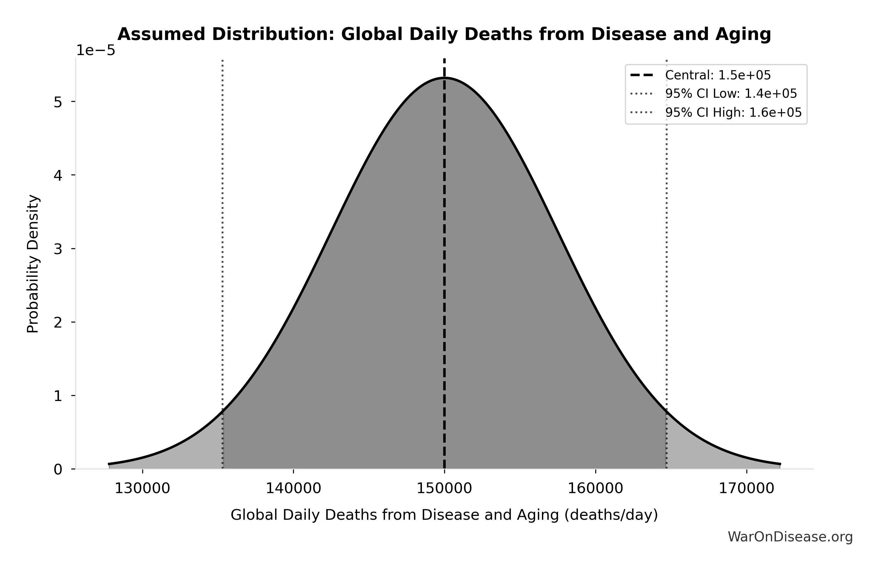
This chart shows the assumed probability distribution for this parameter. The shaded region represents the 95% confidence interval where we expect the true value to fall.
✓ High confidence
YLD Proportion of Total DALYs: 0.39 proportion
Note📊 Details
Proportion of global DALYs that are YLD (years lived with disability) vs YLL (years of life lost). From GBD 2021: 1.13B YLD out of 2.88B total DALYs = 39%.
Source:35
Uncertainty Range
Technical: Distribution: Normal (SE: 0.03 proportion)
Input Distribution
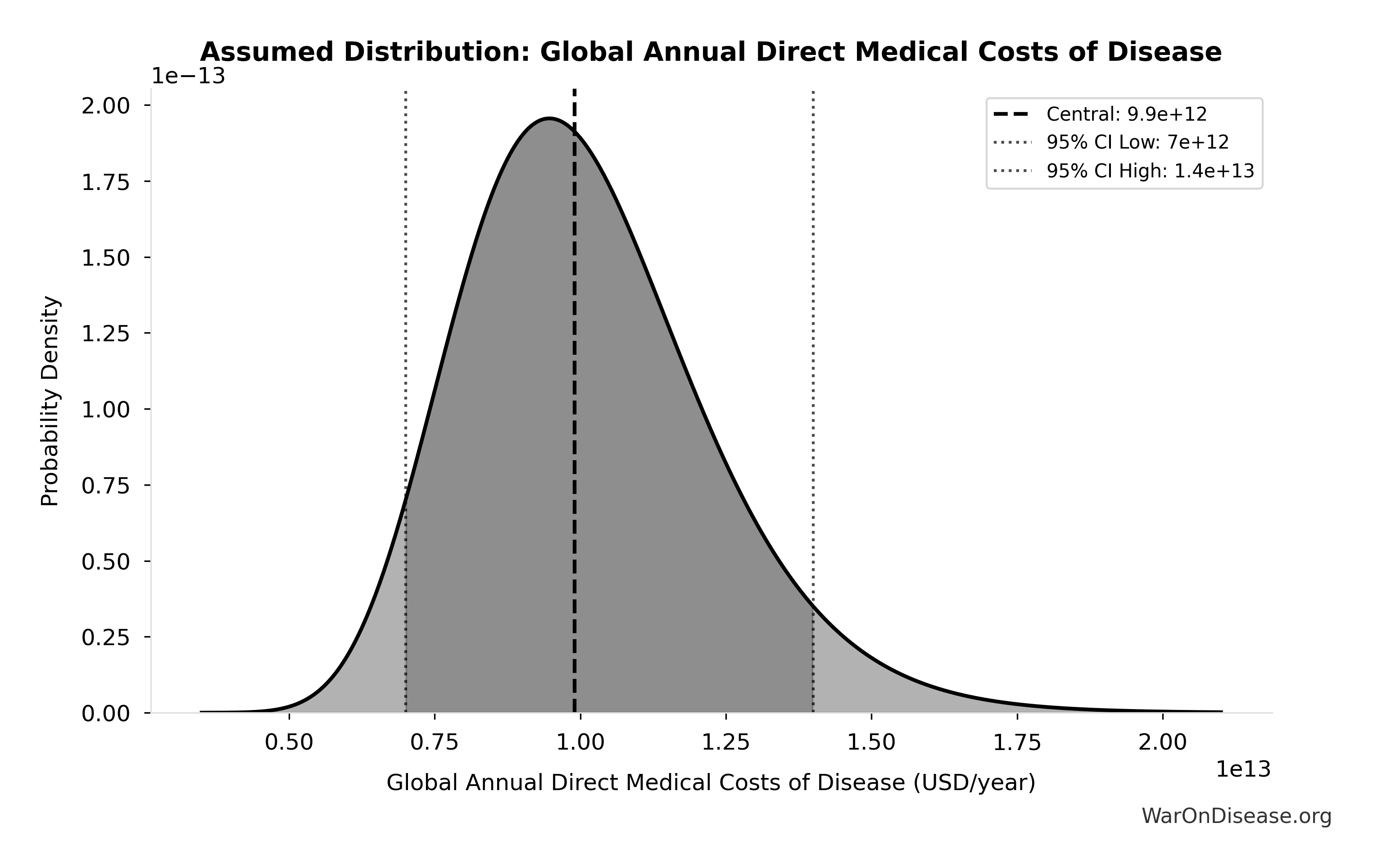
This chart shows the assumed probability distribution for this parameter. The shaded region represents the 95% confidence interval where we expect the true value to fall.
✓ High confidence • 📊 Peer-reviewed
Human Interactome Targeted by Drugs: 12%
Note📊 Details
Percentage of human interactome (protein-protein interactions) targeted by drugs
Source:60
✓ High confidence
Diseases Getting First Treatment Per Year: 15 diseases/year
Note📊 Details
Number of diseases that receive their FIRST effective treatment each year under current system. ~9 rare diseases/year (based on 40 years of ODA: 350 with treatment ÷ 40 years), plus ~5-10 common diseases. Note: FDA approves ~50 drugs/year, but most are for diseases that already have treatments.
Source:68
Uncertainty Range
Technical: 95% CI: [8 diseases/year, 30 diseases/year] • Distribution: Lognormal
What this means: This estimate is highly uncertain. The true value likely falls between 8 diseases/year and 30 diseases/year (±73%). This represents a very wide range that our Monte Carlo simulations account for when calculating overall uncertainty in the results.
The lognormal distribution means values can’t go negative and have a longer tail toward higher values (common for costs and populations).
Input Distribution
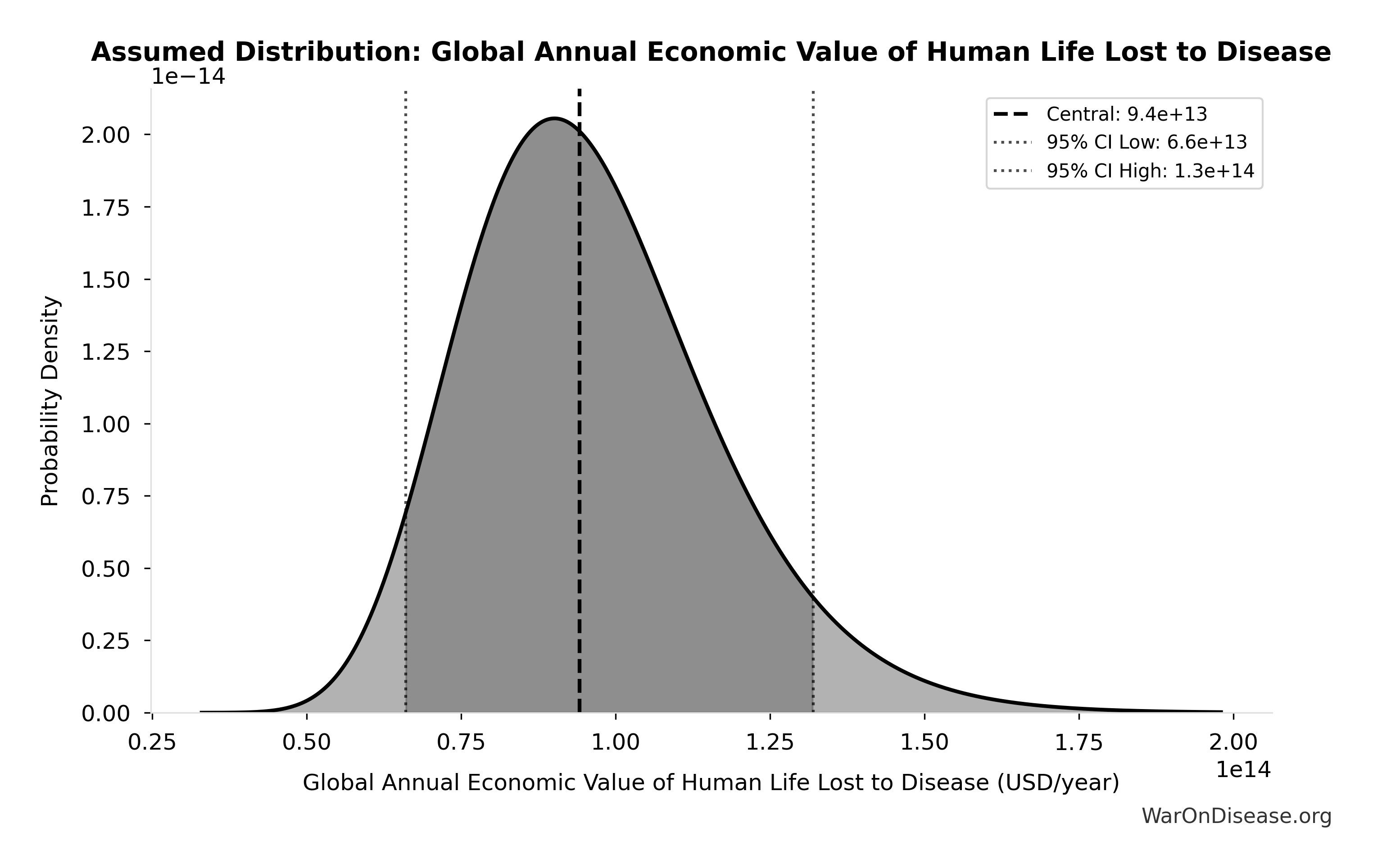
This chart shows the assumed probability distribution for this parameter. The shaded region represents the 95% confidence interval where we expect the true value to fall.
? Low confidence
NIH Standard Research Cost per QALY: $50K
Note📊 Details
Typical cost per QALY for standard NIH-funded medical research portfolio. Reflects the inefficiency of traditional RCTs and basic research-heavy allocation. See confidence_interval for range; ICER uses higher thresholds for value-based pricing.
Source:71
Uncertainty Range
Technical: 95% CI: [$20K, $100K] • Distribution: Lognormal
What this means: This estimate is highly uncertain. The true value likely falls between $20K and $100K (±80%). This represents a very wide range that our Monte Carlo simulations account for when calculating overall uncertainty in the results.
The lognormal distribution means values can’t go negative and have a longer tail toward higher values (common for costs and populations).
Input Distribution

This chart shows the assumed probability distribution for this parameter. The shaded region represents the 95% confidence interval where we expect the true value to fall.
~ Medium confidence
Patient Willingness to Participate in Clinical Trials: 44.8%
Note📊 Details
Patient willingness to participate in drug trials (44.8% in surveys, 88% when actually approached)
Source:73
Uncertainty Range
Technical: 95% CI: [40%, 50%] • Distribution: Normal (SE: 2.5%)
What this means: This estimate has moderate uncertainty. The true value likely falls between 40% and 50% (±11%). This represents a reasonable range that our Monte Carlo simulations account for when calculating overall uncertainty in the results.
The normal distribution means values cluster around the center with equal chances of being higher or lower.
Input Distribution
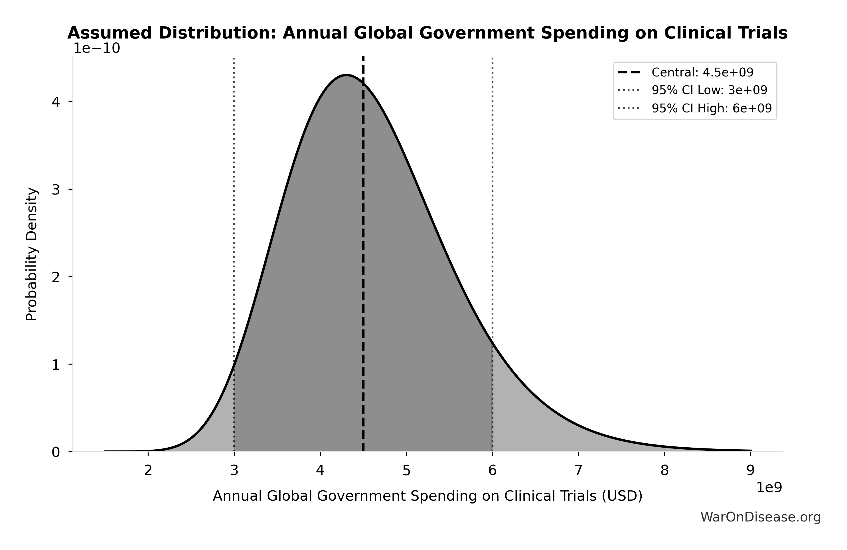
This chart shows the assumed probability distribution for this parameter. The shaded region represents the 95% confidence interval where we expect the true value to fall.
~ Medium confidence
Pharma Drug Development Cost (Current System): $2.6B
Note📊 Details
Average cost to develop one drug in current system
Source:74
Uncertainty Range
Technical: 95% CI: [$1.5B, $4B] • Distribution: Lognormal (SE: $500M)
What this means: There’s significant uncertainty here. The true value likely falls between $1.5B and $4B (±48%). This represents a wide range that our Monte Carlo simulations account for when calculating overall uncertainty in the results.
The lognormal distribution means values can’t go negative and have a longer tail toward higher values (common for costs and populations).
Input Distribution
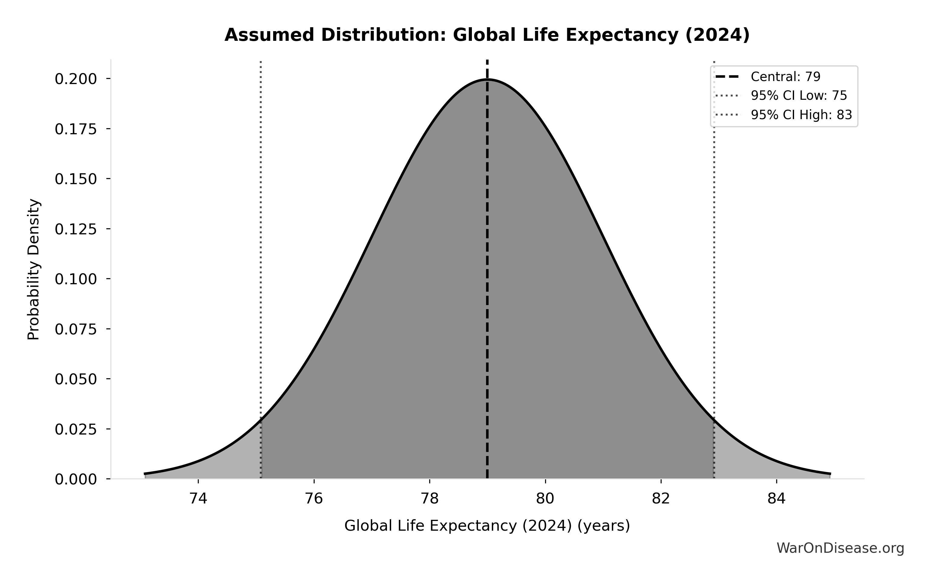
This chart shows the assumed probability distribution for this parameter. The shaded region represents the 95% confidence interval where we expect the true value to fall.
✓ High confidence • 📊 Peer-reviewed
Phase I Safety Trial Duration: 2.3 years
Note📊 Details
Pragmatic Trial Median Cost per Patient (PMC Review): $97
Note📊 Details
Median cost per patient in embedded pragmatic clinical trials (Ramsberg & Platt 2018: 108 trials reviewed, 64 with cost data). IQR: $19-$478 (2015 USD).
Source:80
Uncertainty Range
Technical: 95% CI: [$19, $478] • Distribution: Lognormal
What this means: This estimate is highly uncertain. The true value likely falls between $19 and $478 (±237%). This represents a very wide range that our Monte Carlo simulations account for when calculating overall uncertainty in the results.
The lognormal distribution means values can’t go negative and have a longer tail toward higher values (common for costs and populations).
Input Distribution

This chart shows the assumed probability distribution for this parameter. The shaded region represents the 95% confidence interval where we expect the true value to fall.
✓ High confidence
Global Lead Poisoning Cost: $6T
Note📊 Details
Global cost of lead exposure: World Bank/Lancet estimate. 765 million IQ points lost annually, 5.5 million premature CVD deaths. Cost to eliminate lead from paint, spices, batteries is trivial compared to damage. This is an arbitrage opportunity of immense scale that governance has failed to execute.
Source:47
Uncertainty Range
Technical: 95% CI: [$4T, $8T] • Distribution: Normal (SE: $1T)
What this means: There’s significant uncertainty here. The true value likely falls between $4T and $8T (±33%). This represents a wide range that our Monte Carlo simulations account for when calculating overall uncertainty in the results.
The normal distribution means values cluster around the center with equal chances of being higher or lower.
Input Distribution
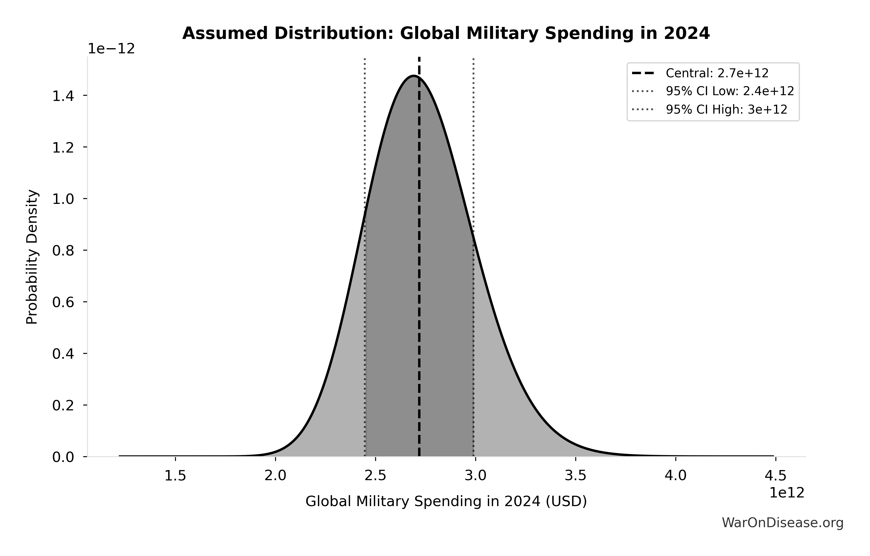
This chart shows the assumed probability distribution for this parameter. The shaded region represents the 95% confidence interval where we expect the true value to fall.
✓ High confidence
Global Migration Opportunity Cost: $57T
Note📊 Details
Unrealized output from migration restrictions. Clemens (2011) calculated eliminating labor mobility barriers could increase global GDP by 50-150%. At $115T global GDP, lower bound = $57T; upper bound = $170T. Even 5% workforce mobility would generate trillions, exceeding all foreign aid ever given. This is the largest single distortion in the global economy.
Source:47
Uncertainty Range
Technical: 95% CI: [$57T, $170T] • Distribution: Lognormal (SE: $30T)
What this means: This estimate is highly uncertain. The true value likely falls between $57T and $170T (±99%). This represents a very wide range that our Monte Carlo simulations account for when calculating overall uncertainty in the results.
The lognormal distribution means values can’t go negative and have a longer tail toward higher values (common for costs and populations).
Input Distribution
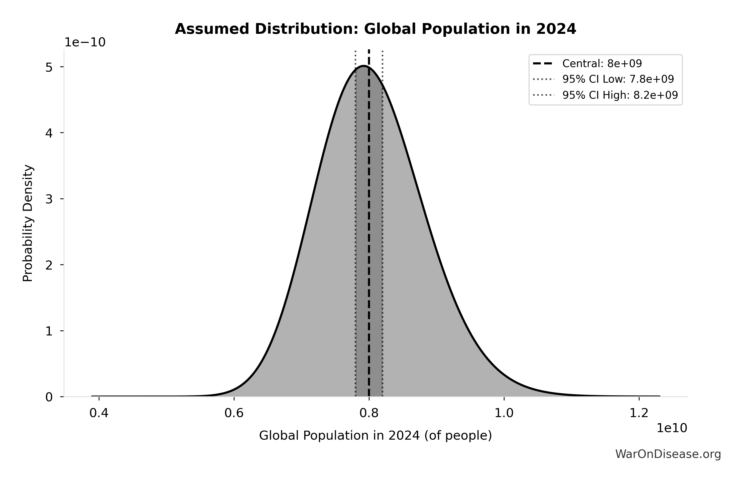
This chart shows the assumed probability distribution for this parameter. The shaded region represents the 95% confidence interval where we expect the true value to fall.
? Low confidence
Global Science Opportunity Cost: $4T
Note📊 Details
Annual opportunity cost from underfunding high-ROI science (fusion, AI safety). Human Genome Project: $3.8B cost, $796B-1T impact (141:1 ROI). Fusion DEMO plant: $5-10B could solve energy/climate permanently. AI safety: <5% of capabilities spending despite existential stakes. Reallocating $200B from military waste at 20x multiplier = $4T foregone growth.
Source:47
Uncertainty Range
Technical: 95% CI: [$2T, $10T] • Distribution: Lognormal (SE: $2T)
What this means: This estimate is highly uncertain. The true value likely falls between $2T and $10T (±100%). This represents a very wide range that our Monte Carlo simulations account for when calculating overall uncertainty in the results.
The lognormal distribution means values can’t go negative and have a longer tail toward higher values (common for costs and populations).
Input Distribution
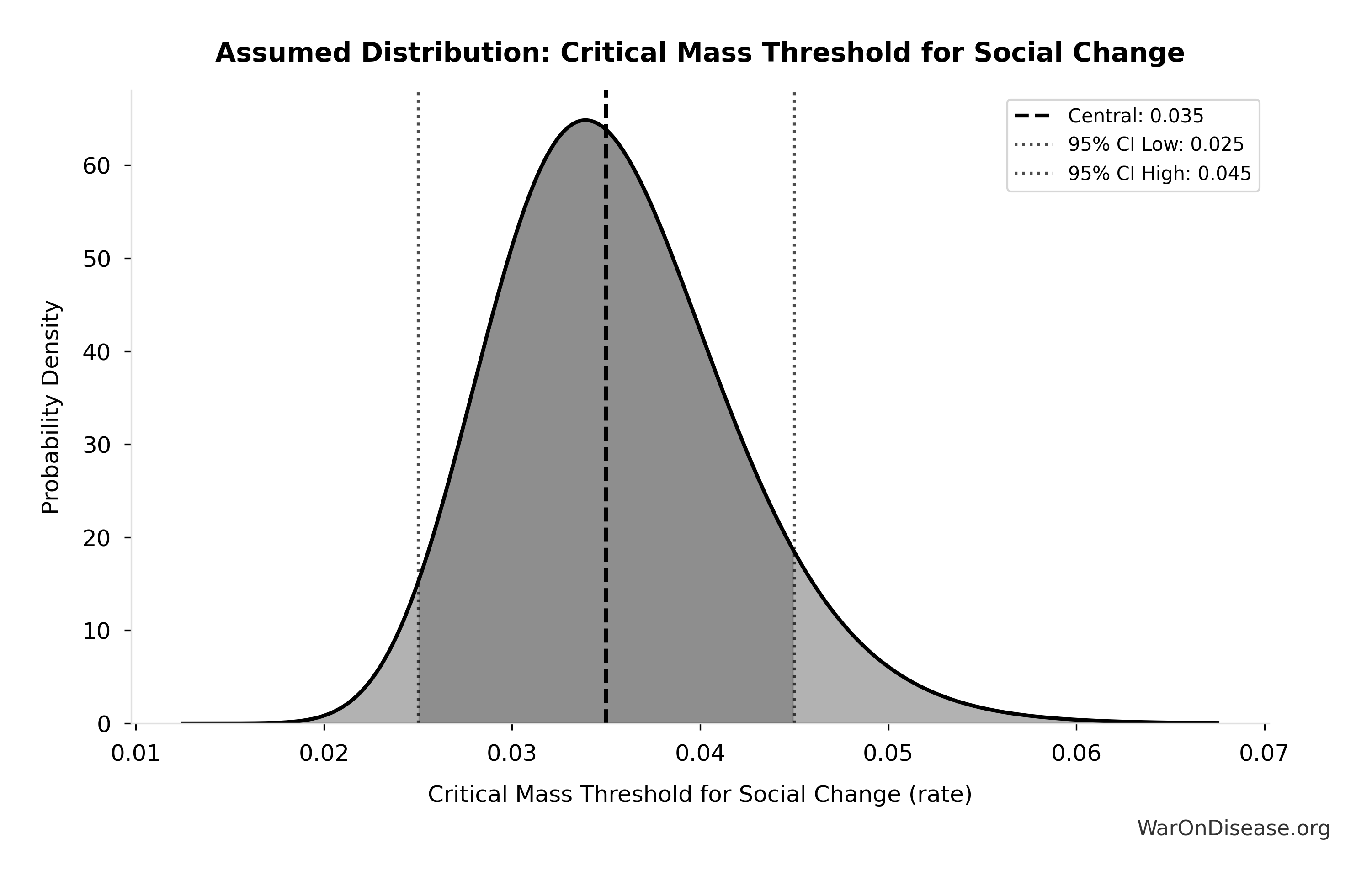
This chart shows the assumed probability distribution for this parameter. The shaded region represents the 95% confidence interval where we expect the true value to fall.
? Low confidence
Political Success Probability: 1%
Note📊 Details
Estimated probability of treaty ratification and sustained implementation. Central estimate 1% is conservative. This assumes 99% chance of failure.
Source:82
Uncertainty Range
Technical: 95% CI: [0.1%, 10%] • Distribution: Beta (SE: 2%)
What this means: This estimate is highly uncertain. The true value likely falls between 0.1% and 10% (±495%). This represents a very wide range that our Monte Carlo simulations account for when calculating overall uncertainty in the results.
The beta distribution means values are bounded and can skew toward one end.
Input Distribution
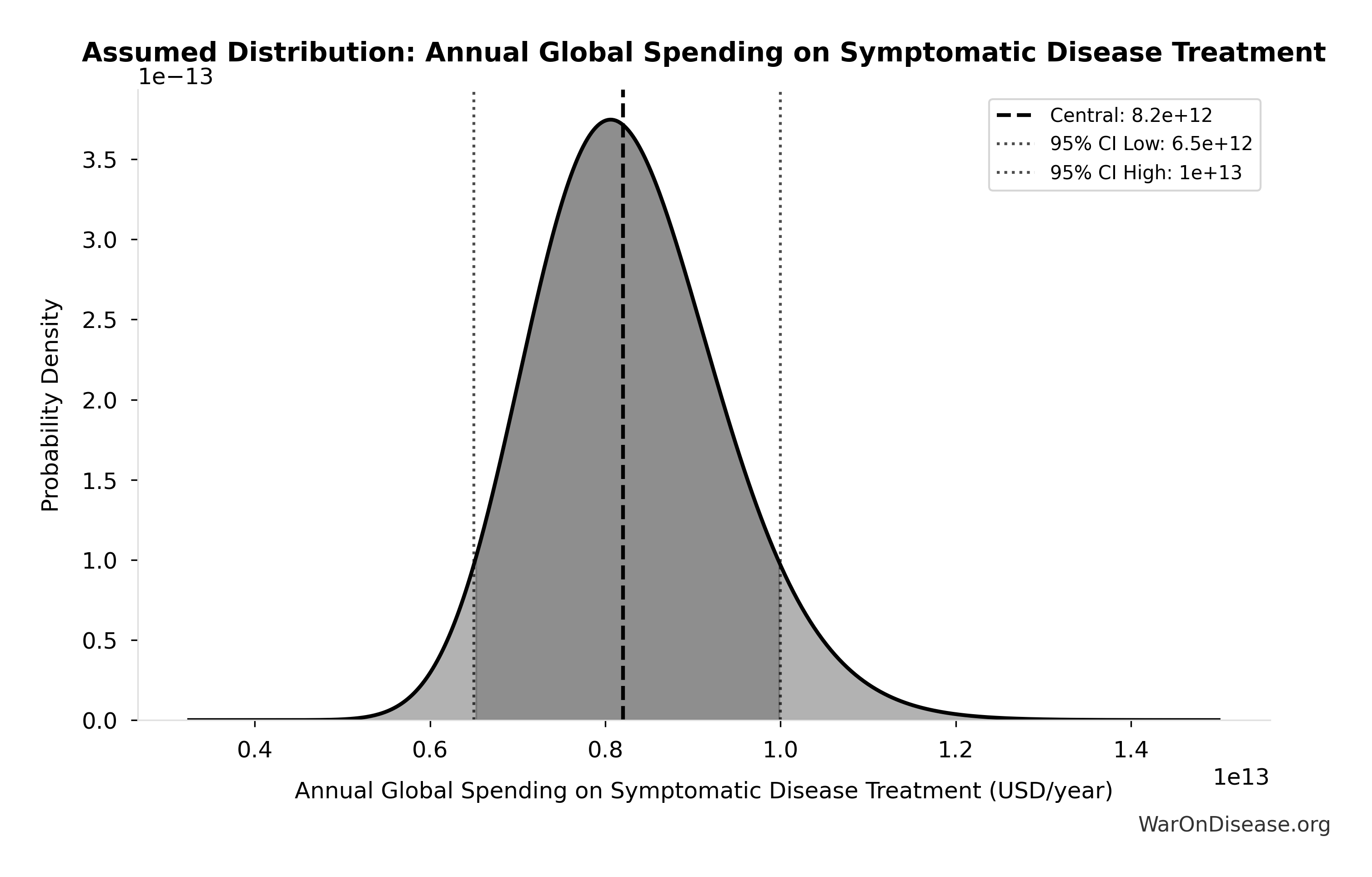
This chart shows the assumed probability distribution for this parameter. The shaded region represents the 95% confidence interval where we expect the true value to fall.
? Low confidence
Pre-1962 Drug Development Cost (2024 Dollars): $24.7M
Note📊 Details
Pre-1962 drug development cost adjusted to 2024 dollars ($6.5M × 3.80 = $24.7M, CPI-adjusted from Baily 1972)
Source:85
Uncertainty Range
Technical: 95% CI: [$19.5M, $30M] • Distribution: Lognormal
What this means: This estimate has moderate uncertainty. The true value likely falls between $19.5M and $30M (±21%). This represents a reasonable range that our Monte Carlo simulations account for when calculating overall uncertainty in the results.
The lognormal distribution means values can’t go negative and have a longer tail toward higher values (common for costs and populations).
Input Distribution
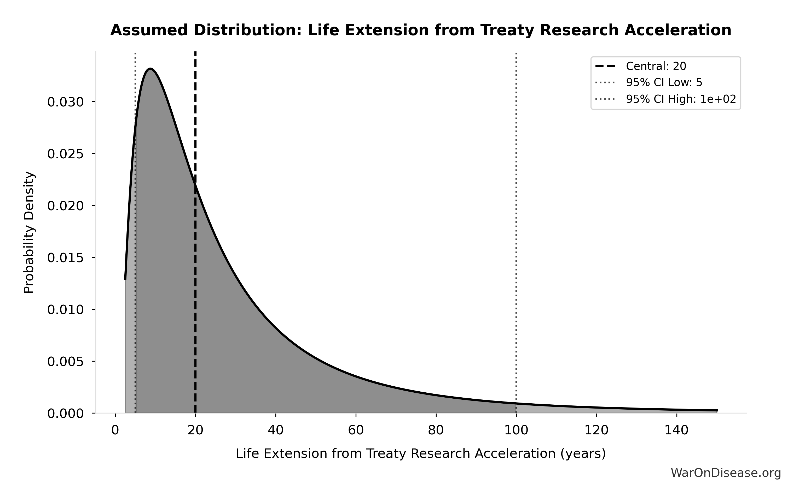
This chart shows the assumed probability distribution for this parameter. The shaded region represents the 95% confidence interval where we expect the true value to fall.
✓ High confidence • 📊 Peer-reviewed
Pre-1962 Physician Count (Unverified): 144 thousand physicians
Note📊 Details
Estimated physicians conducting real-world efficacy trials pre-1962 (unverified estimate)
Source:86
? Low confidence
Total Number of Rare Diseases Globally: 7 thousand diseases
Note📊 Details
Total number of rare diseases globally
Source:87
Uncertainty Range
Technical: 95% CI: [6 thousand diseases, 10 thousand diseases] • Distribution: Normal
What this means: There’s significant uncertainty here. The true value likely falls between 6 thousand diseases and 10 thousand diseases (±29%). This represents a wide range that our Monte Carlo simulations account for when calculating overall uncertainty in the results.
The normal distribution means values cluster around the center with equal chances of being higher or lower.
Input Distribution
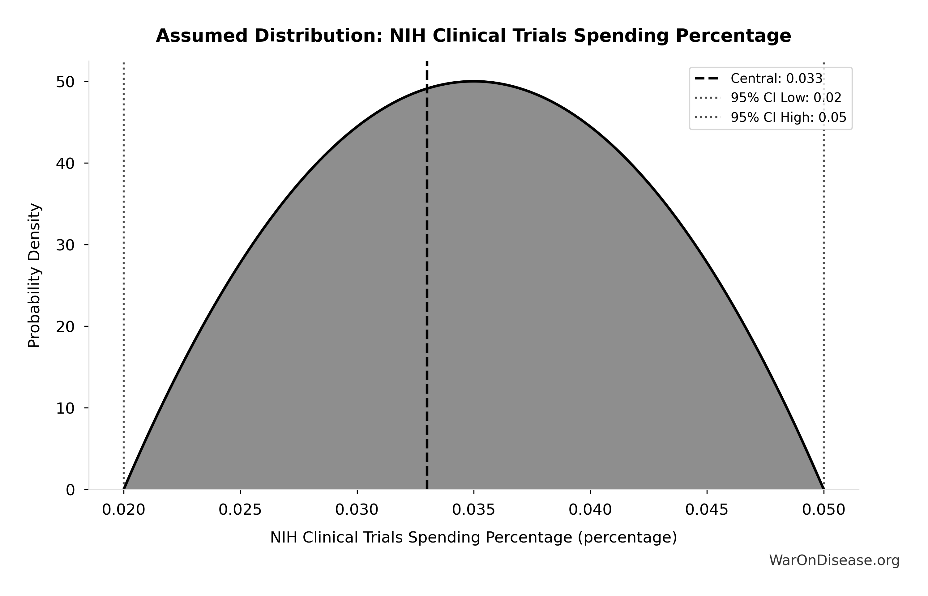
This chart shows the assumed probability distribution for this parameter. The shaded region represents the 95% confidence interval where we expect the true value to fall.
✓ High confidence
Recovery Trial Cost per Patient: $500
Note📊 Details
RECOVERY trial cost per patient. Note: RECOVERY was an outlier - hospital-based during COVID emergency, minimal extra procedures, existing NHS infrastructure, streamlined consent. Replicating this globally will be harder.
Source:88
Uncertainty Range
Technical: 95% CI: [$400, $2.5K] • Distribution: Lognormal
What this means: This estimate is highly uncertain. The true value likely falls between $400 and $2.5K (±210%). This represents a very wide range that our Monte Carlo simulations account for when calculating overall uncertainty in the results.
The lognormal distribution means values can’t go negative and have a longer tail toward higher values (common for costs and populations).
Input Distribution
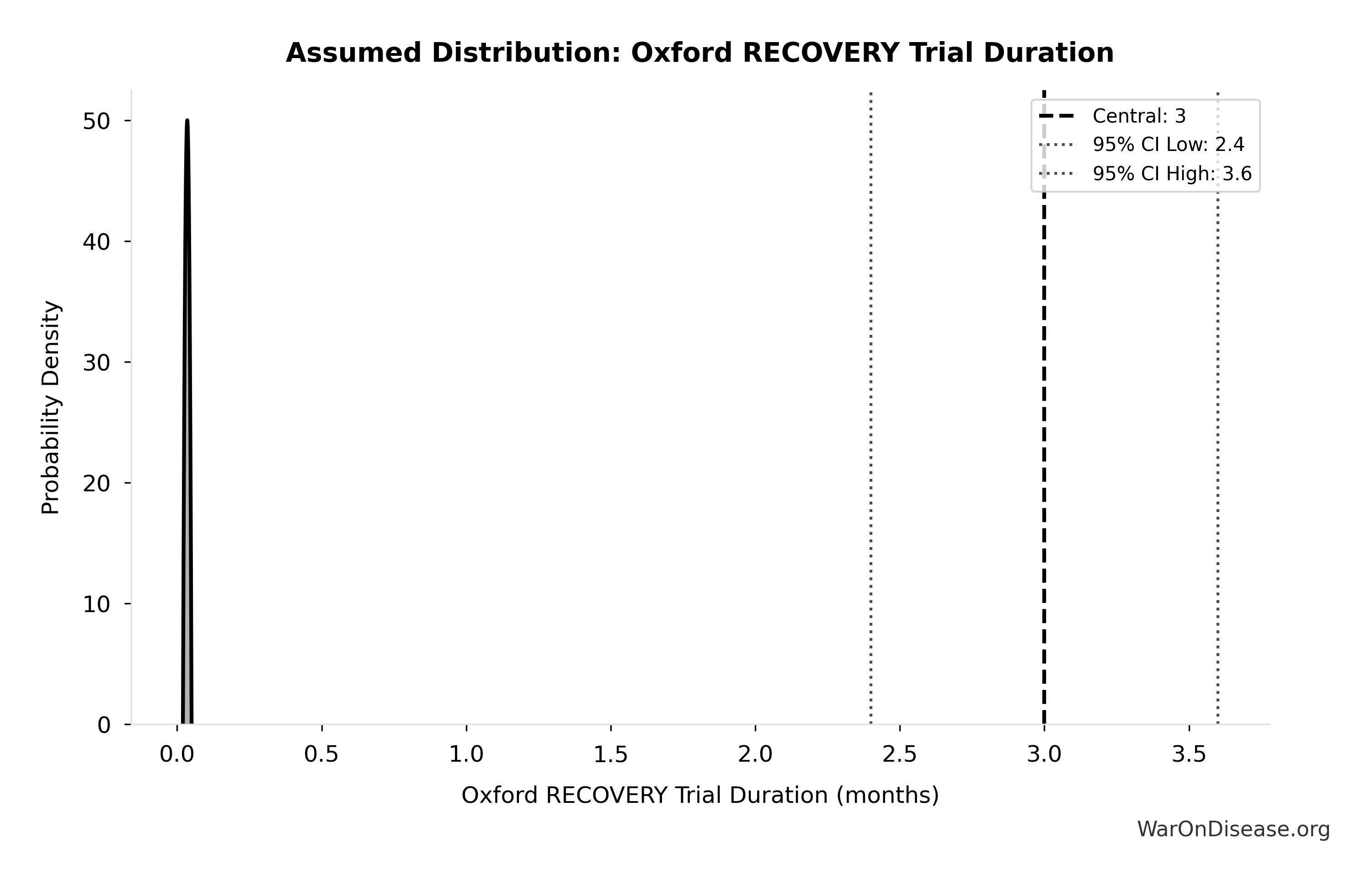
This chart shows the assumed probability distribution for this parameter. The shaded region represents the 95% confidence interval where we expect the true value to fall.
✓ High confidence
RECOVERY Trial Global Lives Saved: 1 million lives
Note📊 Details
Estimated lives saved globally by RECOVERY trial’s dexamethasone discovery. NHS England estimate (March 2021). Based on Águas et al. Nature Communications 2021 methodology applying RECOVERY trial mortality reductions (36% ventilated, 18% oxygen) to global COVID hospitalizations. Wide uncertainty range reflects extrapolation assumptions.
Source:89
Uncertainty Range
Technical: 95% CI: [500 thousand lives, 2 million lives] • Distribution: Lognormal
What this means: This estimate is highly uncertain. The true value likely falls between 500 thousand lives and 2 million lives (±75%). This represents a very wide range that our Monte Carlo simulations account for when calculating overall uncertainty in the results.
The lognormal distribution means values can’t go negative and have a longer tail toward higher values (common for costs and populations).
Input Distribution
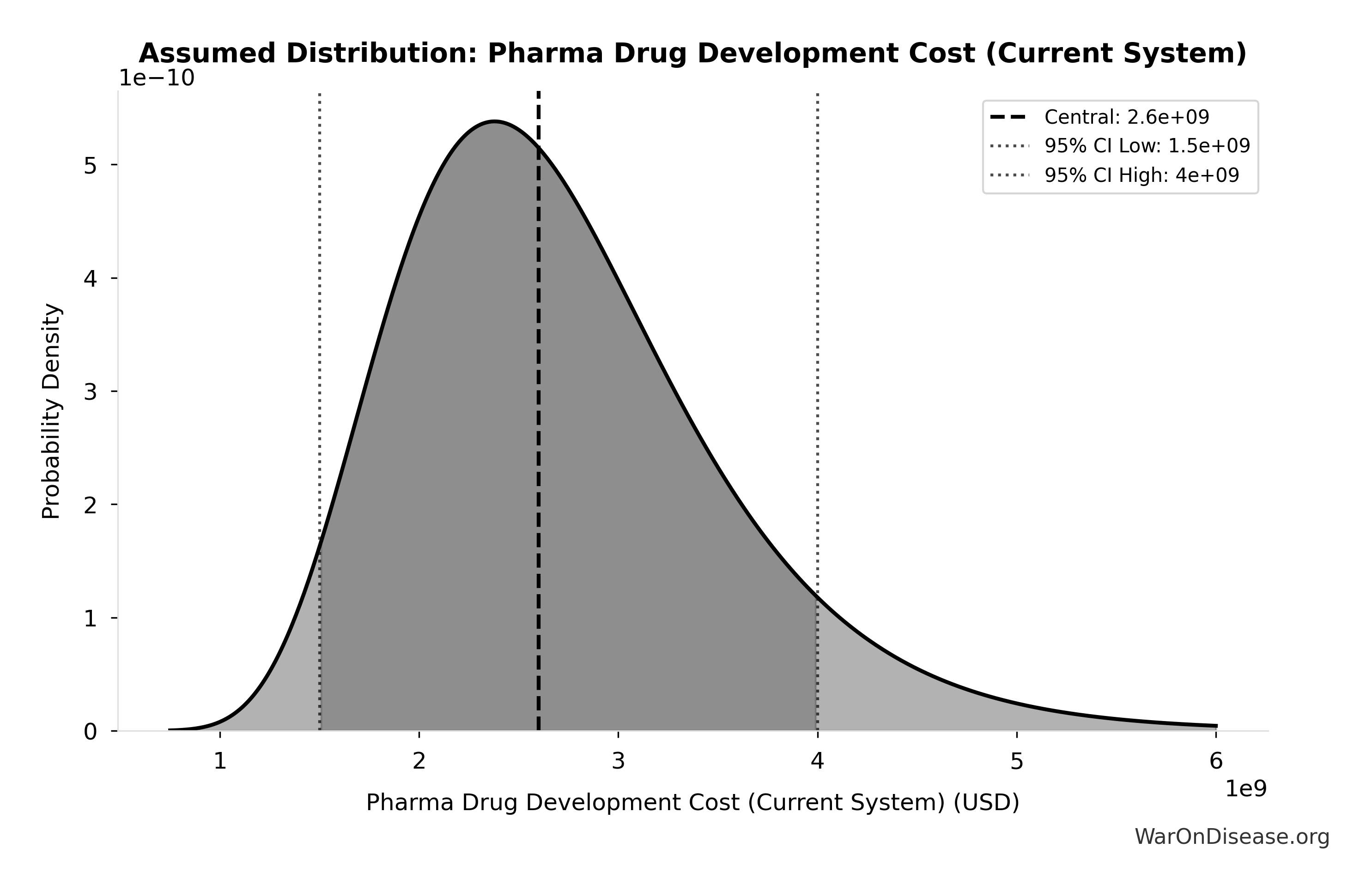
This chart shows the assumed probability distribution for this parameter. The shaded region represents the 95% confidence interval where we expect the true value to fall.
~ Medium confidence
RECOVERY Trial Total Cost: $20M
Note📊 Details
Total cost of UK RECOVERY trial. Enrolled tens of thousands of patients across multiple treatment arms. Discovered dexamethasone reduces COVID mortality by ~1/3 in severe cases.
Source:72
Uncertainty Range
Technical: 95% CI: [$15M, $25M] • Distribution: Lognormal
What this means: This estimate has moderate uncertainty. The true value likely falls between $15M and $25M (±25%). This represents a reasonable range that our Monte Carlo simulations account for when calculating overall uncertainty in the results.
The lognormal distribution means values can’t go negative and have a longer tail toward higher values (common for costs and populations).
Input Distribution
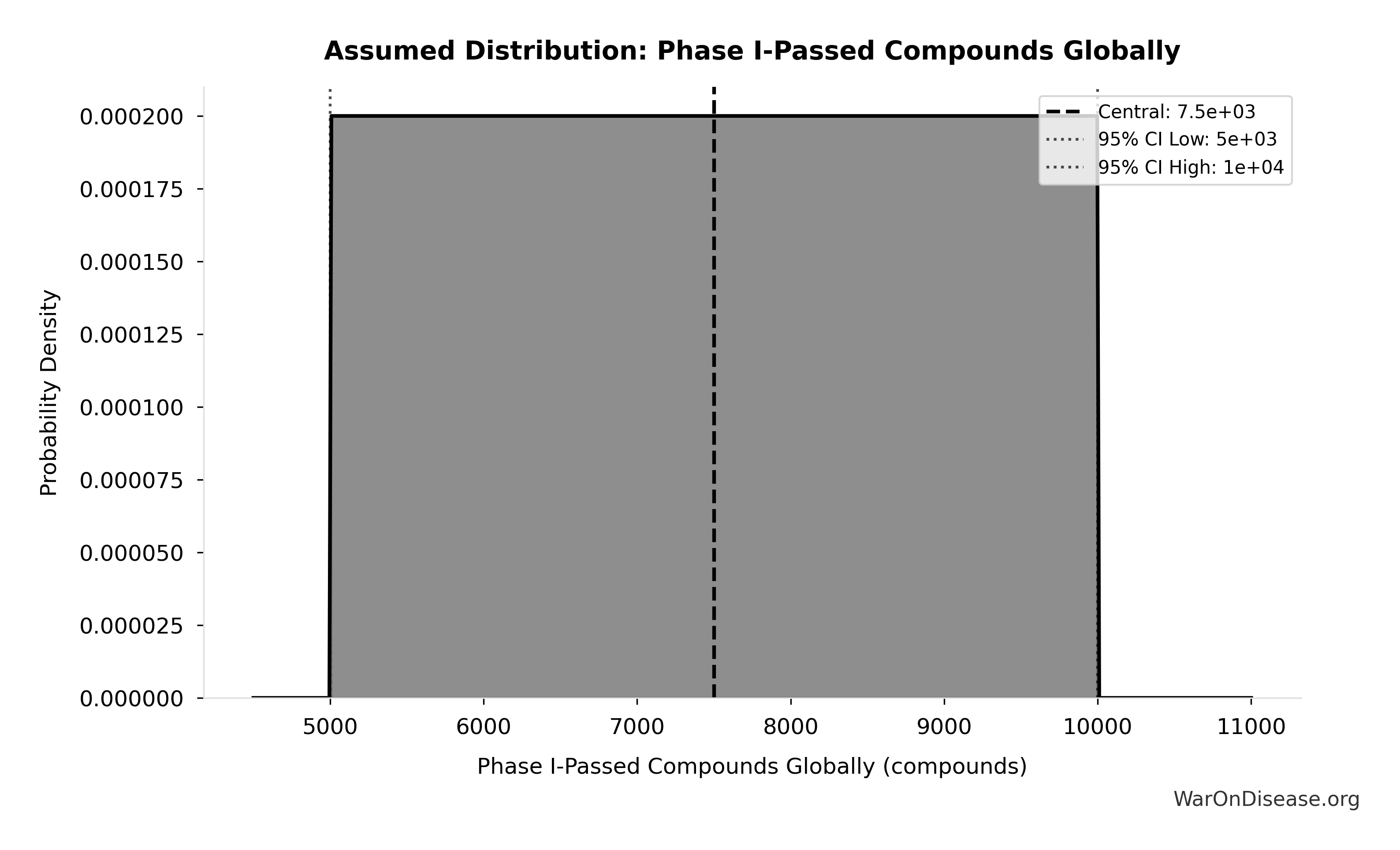
This chart shows the assumed probability distribution for this parameter. The shaded region represents the 95% confidence interval where we expect the true value to fall.
✓ High confidence
Mean Age of Preventable Death from Post-Safety Efficacy Delay: 62 years
Note📊 Details
Mean age of preventable death from post-safety efficacy testing regulatory delay (Phase 2-4)
Source:4
Uncertainty Range
Technical: Distribution: Normal (SE: 3 years)
Input Distribution
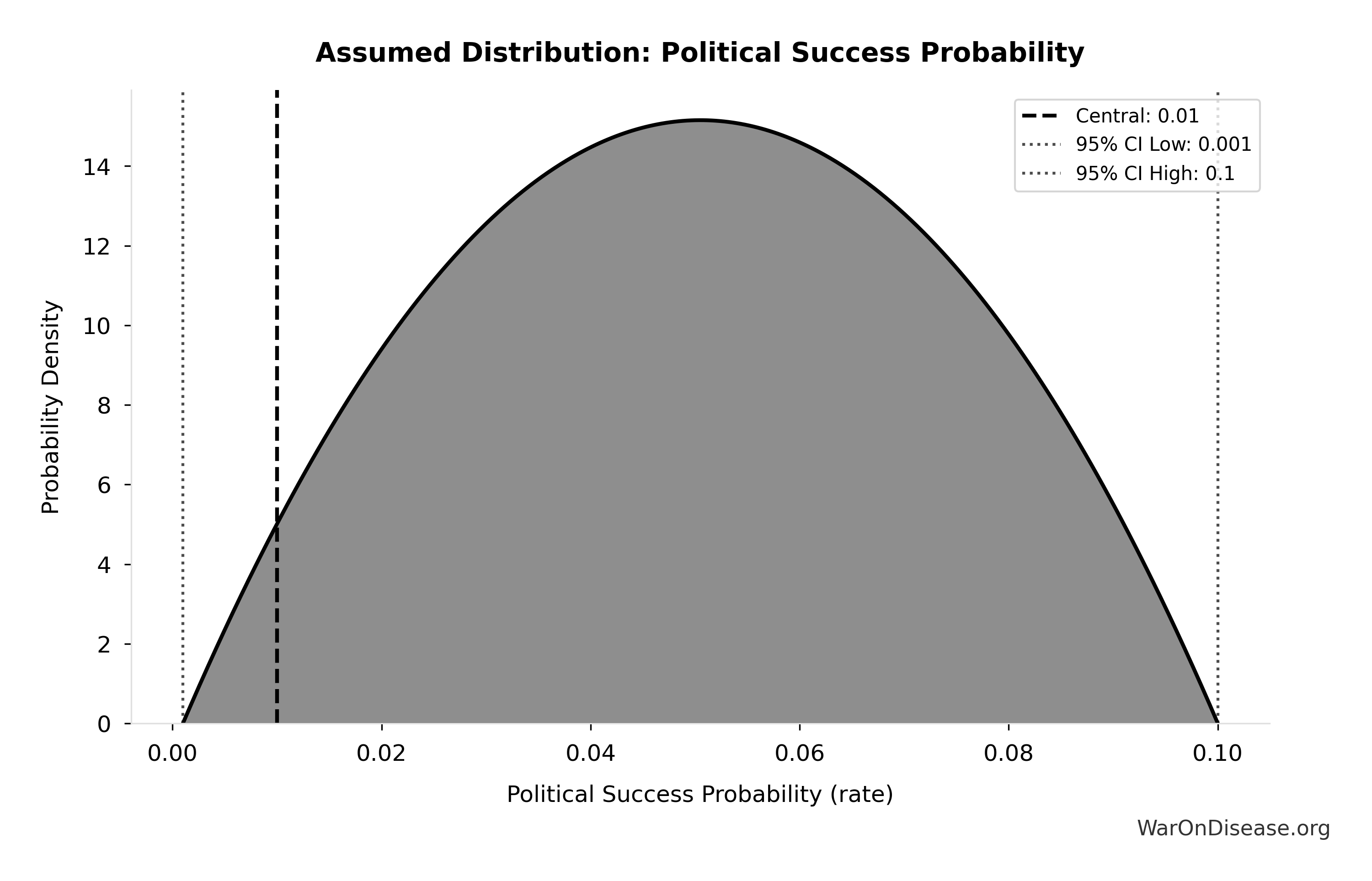
This chart shows the assumed probability distribution for this parameter. The shaded region represents the 95% confidence interval where we expect the true value to fall.
~ Medium confidence • 📊 Peer-reviewed
Pre-Death Suffering Period During Post-Safety Efficacy Delay: 6 years
Note📊 Details
Pre-death suffering period during post-safety efficacy testing delay (average years lived with untreated condition while awaiting Phase 2-4 completion)
Source:4
Uncertainty Range
Technical: 95% CI: [4 years, 9 years] • Distribution: Lognormal
What this means: There’s significant uncertainty here. The true value likely falls between 4 years and 9 years (±42%). This represents a wide range that our Monte Carlo simulations account for when calculating overall uncertainty in the results.
The lognormal distribution means values can’t go negative and have a longer tail toward higher values (common for costs and populations).
Input Distribution
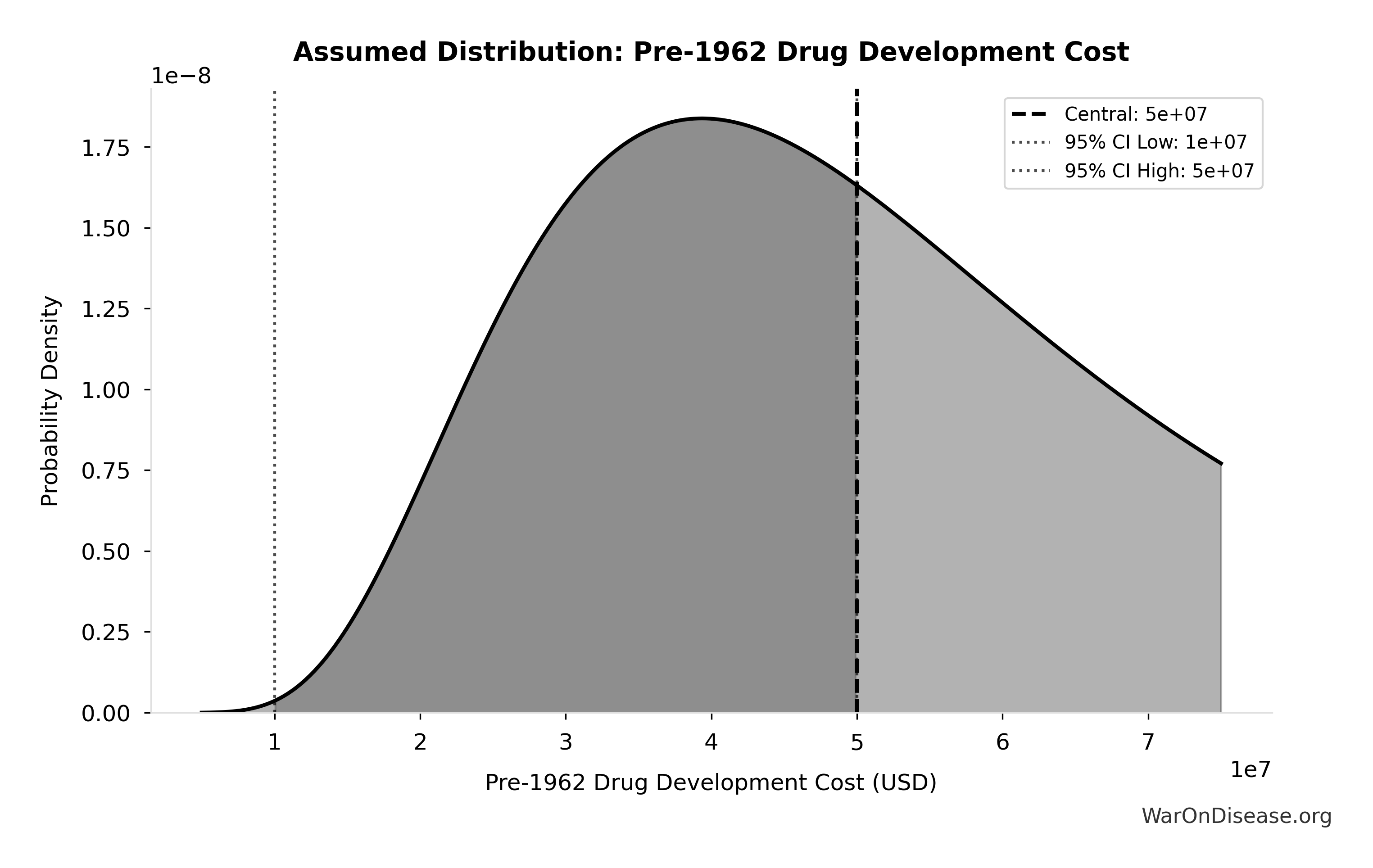
This chart shows the assumed probability distribution for this parameter. The shaded region represents the 95% confidence interval where we expect the true value to fall.
~ Medium confidence • 📊 Peer-reviewed
Return on Investment from Smallpox Eradication Campaign: 280:1
Note📊 Details
Standard Economic Value per QALY: $150K
Note📊 Details
Standard economic value per QALY
Source:96
Uncertainty Range
Technical: Distribution: Normal (SE: $30K)
Input Distribution
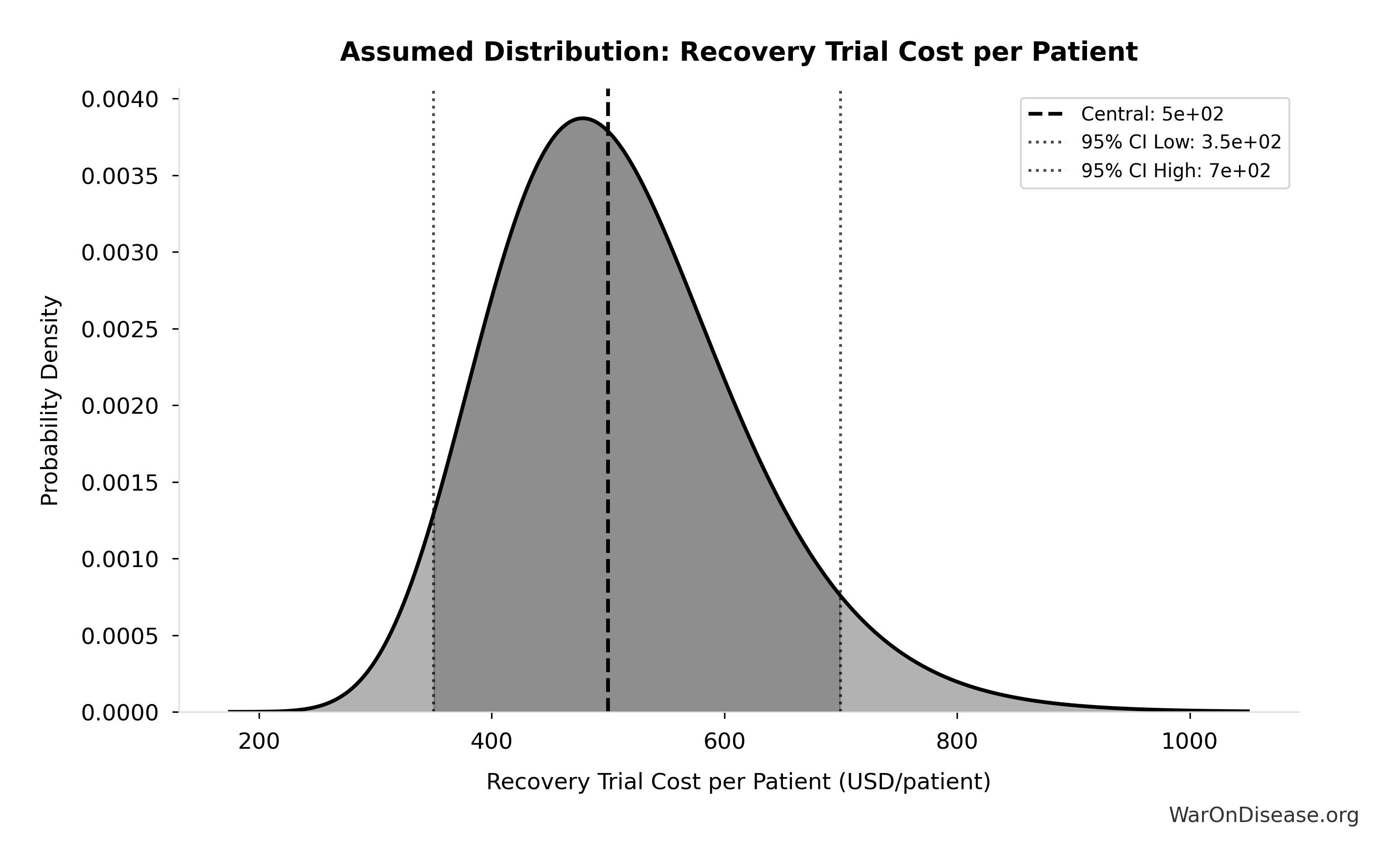
This chart shows the assumed probability distribution for this parameter. The shaded region represents the 95% confidence interval where we expect the true value to fall.
✓ High confidence
Deaths from 9/11 Terrorist Attacks: 3 thousand deaths
Note📊 Details
Deaths from 9/11 terrorist attacks
Source:102
Uncertainty Range
Technical: Distribution: Fixed
✓ High confidence
Thalidomide Cases Worldwide: 15 thousand cases
Note📊 Details
Total thalidomide birth defect cases worldwide (1957-1962)
Source:103
Uncertainty Range
Technical: 95% CI: [10 thousand cases, 20 thousand cases] • Distribution: Lognormal
What this means: There’s significant uncertainty here. The true value likely falls between 10 thousand cases and 20 thousand cases (±33%). This represents a wide range that our Monte Carlo simulations account for when calculating overall uncertainty in the results.
The lognormal distribution means values can’t go negative and have a longer tail toward higher values (common for costs and populations).
Input Distribution
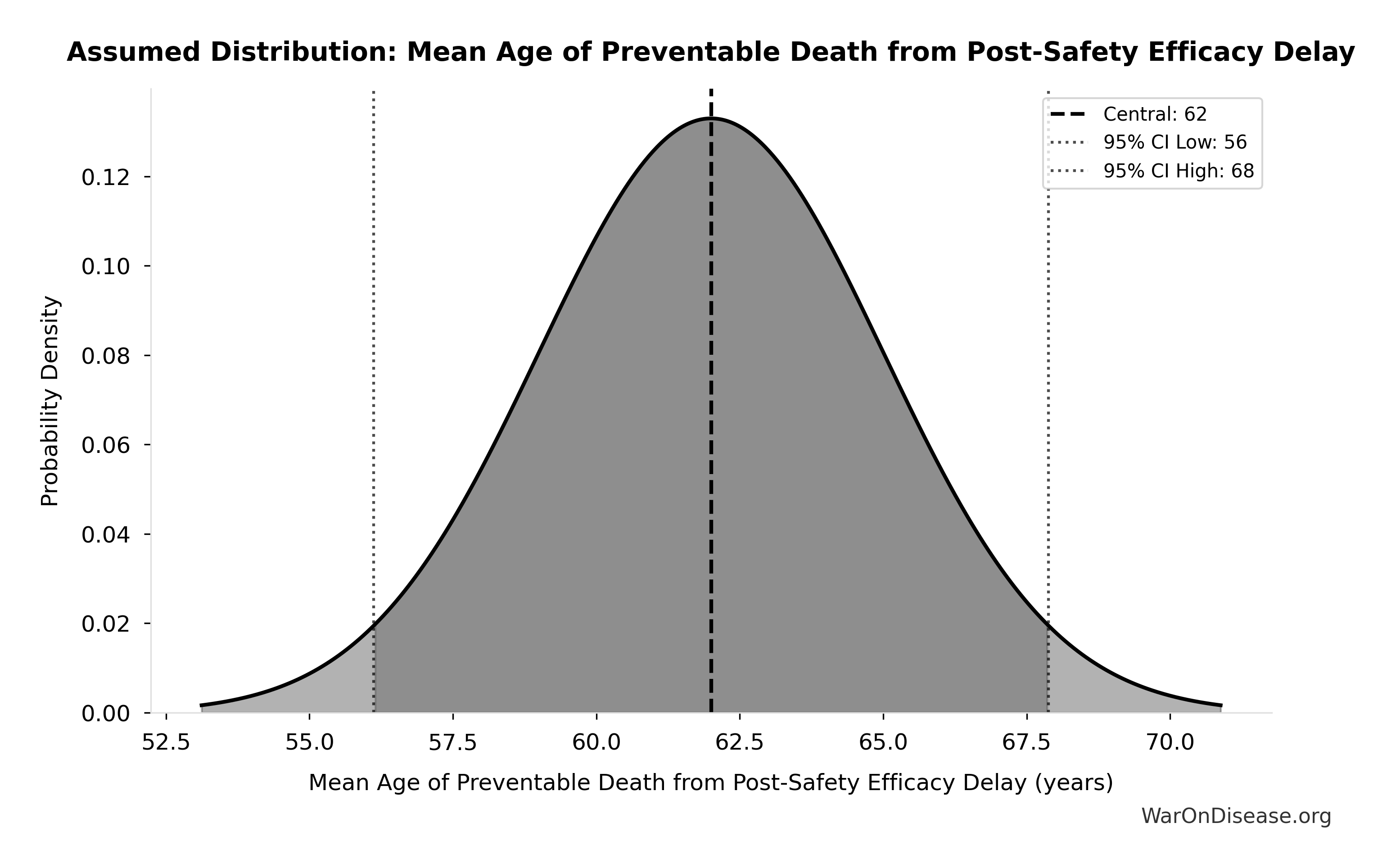
This chart shows the assumed probability distribution for this parameter. The shaded region represents the 95% confidence interval where we expect the true value to fall.
~ Medium confidence
Thalidomide Disability Weight: 0.4:1
Note📊 Details
Disability weight for thalidomide survivors (limb deformities, organ damage)
Source:104
Uncertainty Range
Technical: 95% CI: [0.32:1, 0.48:1] • Distribution: Lognormal
What this means: This estimate has moderate uncertainty. The true value likely falls between 0.32:1 and 0.48:1 (±20%). This represents a reasonable range that our Monte Carlo simulations account for when calculating overall uncertainty in the results.
The lognormal distribution means values can’t go negative and have a longer tail toward higher values (common for costs and populations).
Input Distribution
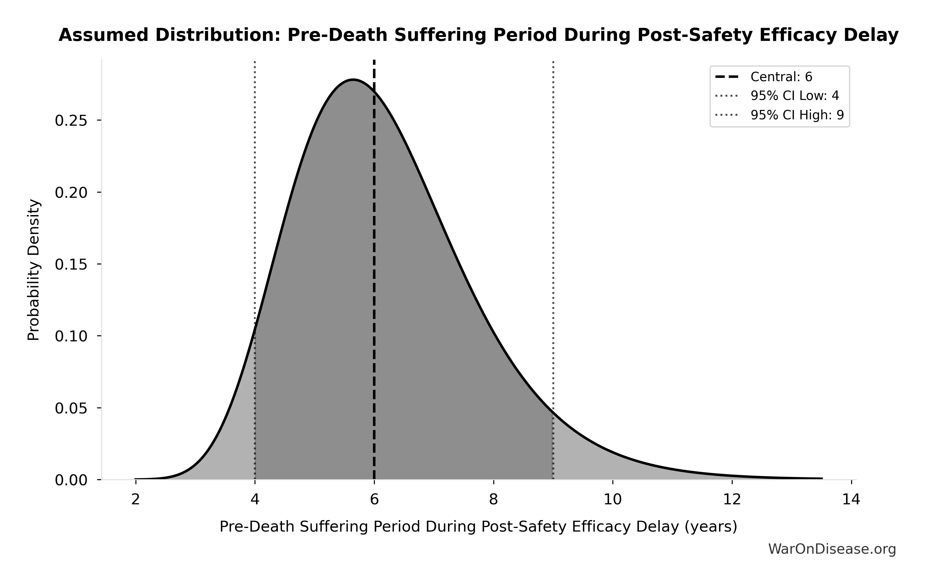
This chart shows the assumed probability distribution for this parameter. The shaded region represents the 95% confidence interval where we expect the true value to fall.
~ Medium confidence
Thalidomide Mortality Rate: 40%
Note📊 Details
Mortality rate for thalidomide-affected infants (died within first year)
Source:103
Uncertainty Range
Technical: 95% CI: [35%, 45%] • Distribution: Lognormal
What this means: This estimate has moderate uncertainty. The true value likely falls between 35% and 45% (±13%). This represents a reasonable range that our Monte Carlo simulations account for when calculating overall uncertainty in the results.
The lognormal distribution means values can’t go negative and have a longer tail toward higher values (common for costs and populations).
Input Distribution
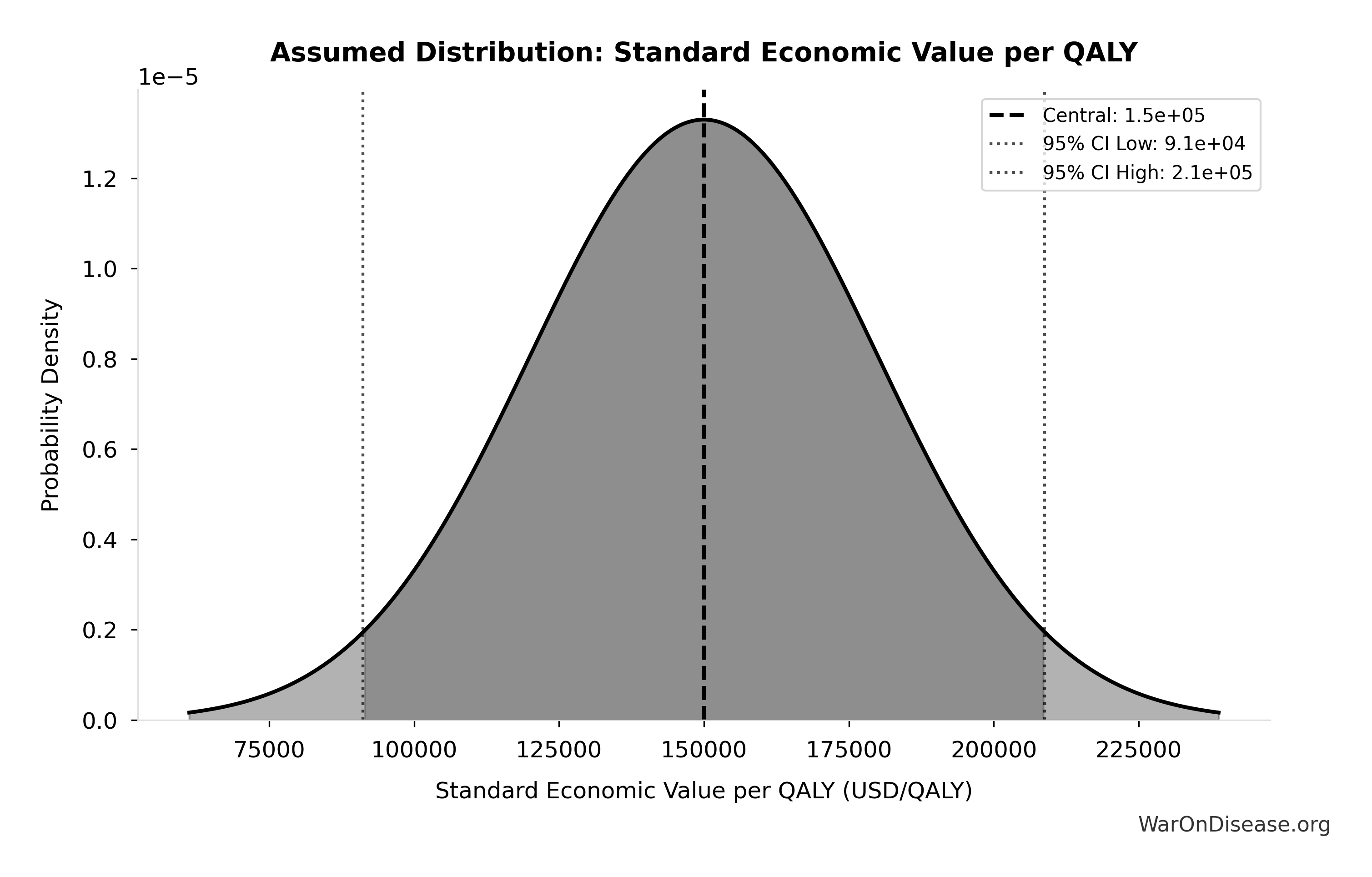
This chart shows the assumed probability distribution for this parameter. The shaded region represents the 95% confidence interval where we expect the true value to fall.
✓ High confidence
Thalidomide Survivor Lifespan: 60 years
Note📊 Details
Average lifespan for thalidomide survivors
Source:104
Uncertainty Range
Technical: 95% CI: [50 years, 70 years] • Distribution: Lognormal
What this means: This estimate has moderate uncertainty. The true value likely falls between 50 years and 70 years (±17%). This represents a reasonable range that our Monte Carlo simulations account for when calculating overall uncertainty in the results.
The lognormal distribution means values can’t go negative and have a longer tail toward higher values (common for costs and populations).
Input Distribution
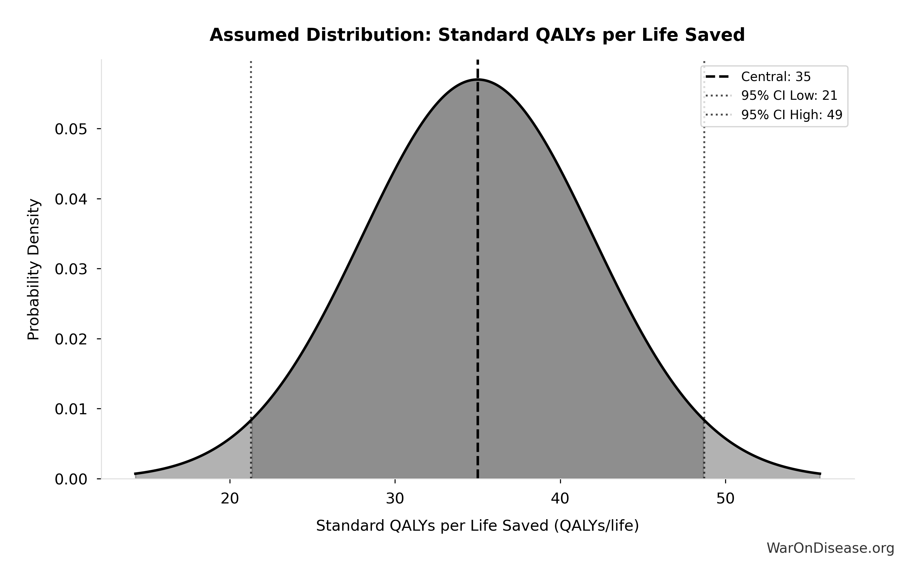
This chart shows the assumed probability distribution for this parameter. The shaded region represents the 95% confidence interval where we expect the true value to fall.
~ Medium confidence
US Population Share 1960: 6%
Note📊 Details
US share of world population in 1960
Source:105
Uncertainty Range
Technical: 95% CI: [5.5%, 6.5%] • Distribution: Lognormal
What this means: We’re quite confident in this estimate. The true value likely falls between 5.5% and 6.5% (±8%). This represents a narrow range that our Monte Carlo simulations account for when calculating overall uncertainty in the results.
The lognormal distribution means values can’t go negative and have a longer tail toward higher values (common for costs and populations).
Input Distribution
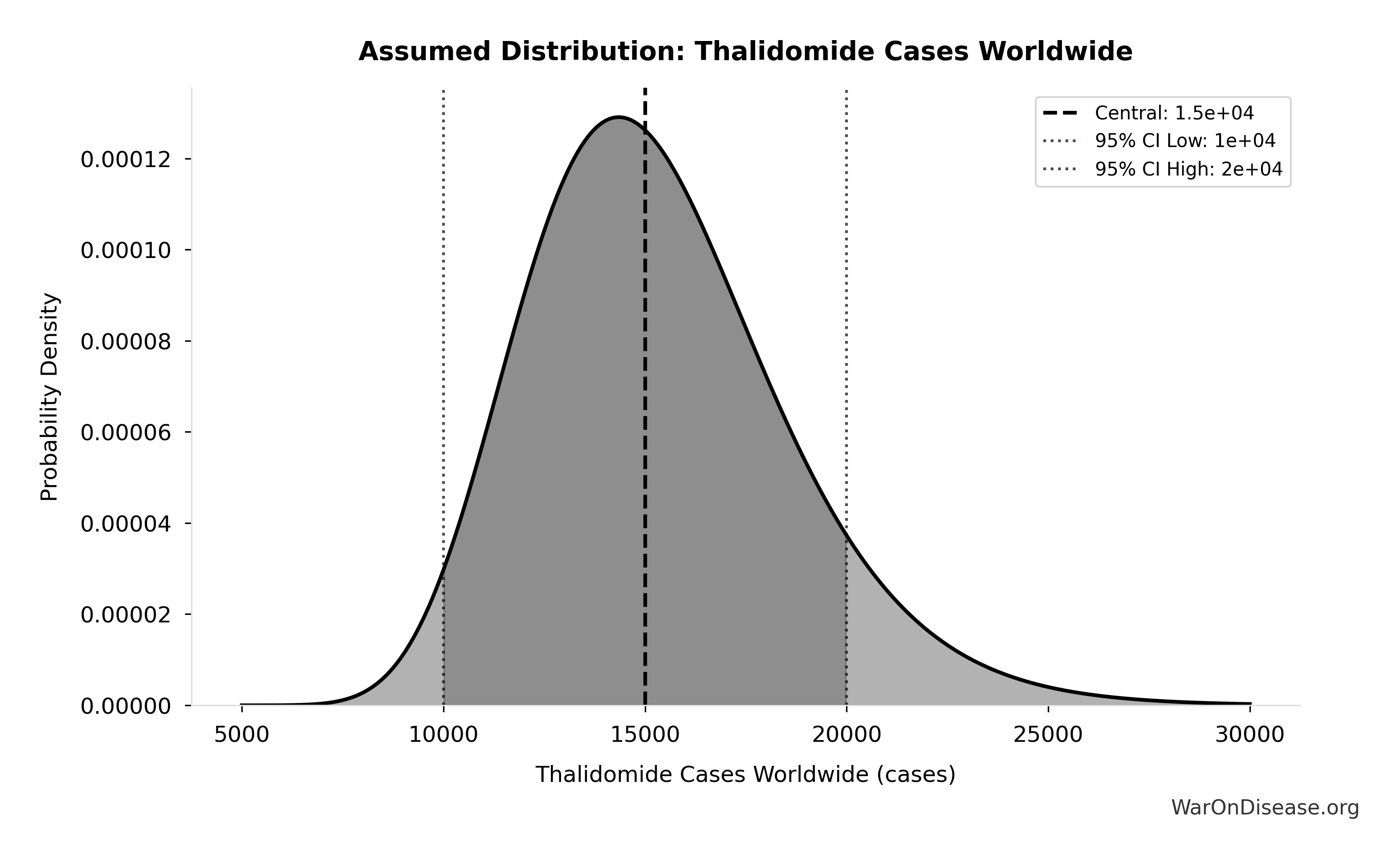
This chart shows the assumed probability distribution for this parameter. The shaded region represents the 95% confidence interval where we expect the true value to fall.
✓ High confidence
Phase 3 Cost per Patient: $41K
Note📊 Details
Phase 3 cost per patient (median from FDA study)
Source:106
Uncertainty Range
Technical: 95% CI: [$20K, $120K] • Distribution: Lognormal
What this means: This estimate is highly uncertain. The true value likely falls between $20K and $120K (±122%). This represents a very wide range that our Monte Carlo simulations account for when calculating overall uncertainty in the results.
The lognormal distribution means values can’t go negative and have a longer tail toward higher values (common for costs and populations).
Input Distribution
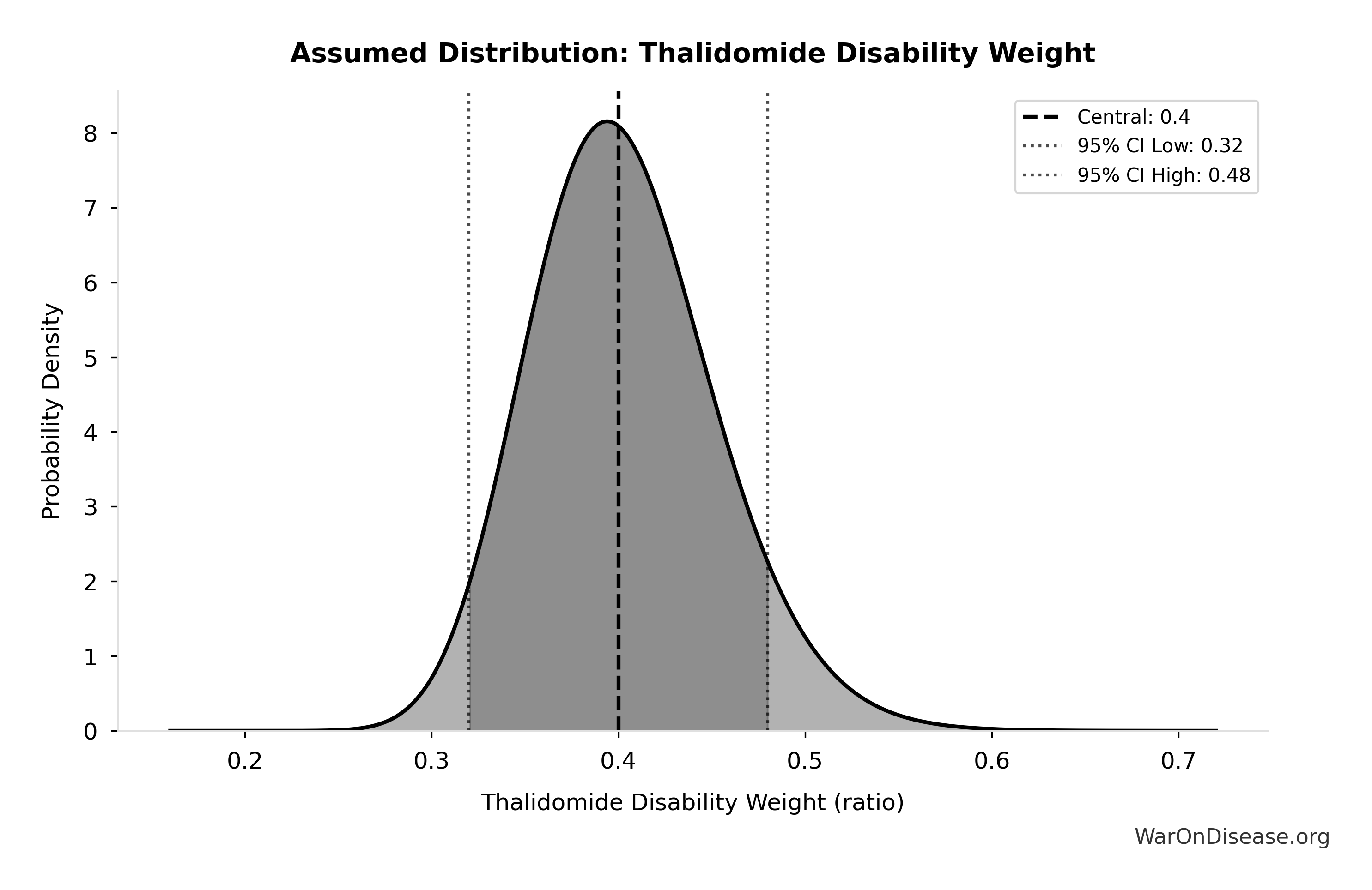
This chart shows the assumed probability distribution for this parameter. The shaded region represents the 95% confidence interval where we expect the true value to fall.
✓ High confidence
US Military Spending at WW2 Peak (Constant 2024 Dollars): $1.42T
Note📊 Details
US military spending at WW2 peak (1945) in constant 2024 dollars
Source:126
Uncertainty Range
Technical: Distribution: Fixed
✓ High confidence
US Military Spending in 1947 (Constant 2024 Dollars): $176B
Note📊 Details
US military spending in 1947 (post-WW2 trough, 2 years after peak) in constant 2024 dollars
Source:126
Uncertainty Range
Technical: Distribution: Fixed
✓ High confidence
Valley of Death Attrition Rate: 40%
Note📊 Details
Percentage of promising Phase 1-passed compounds abandoned primarily due to Phase 2/3 cost barriers (not scientific failure). Conservative estimate: many rare disease, natural compound, and low-margin drugs never tested.
Source:133
Uncertainty Range
Technical: 95% CI: [25%, 55%] • Distribution: Uniform
What this means: There’s significant uncertainty here. The true value likely falls between 25% and 55% (±38%). This represents a wide range that our Monte Carlo simulations account for when calculating overall uncertainty in the results.
The uniform distribution means any value in the range is equally likely.
Input Distribution
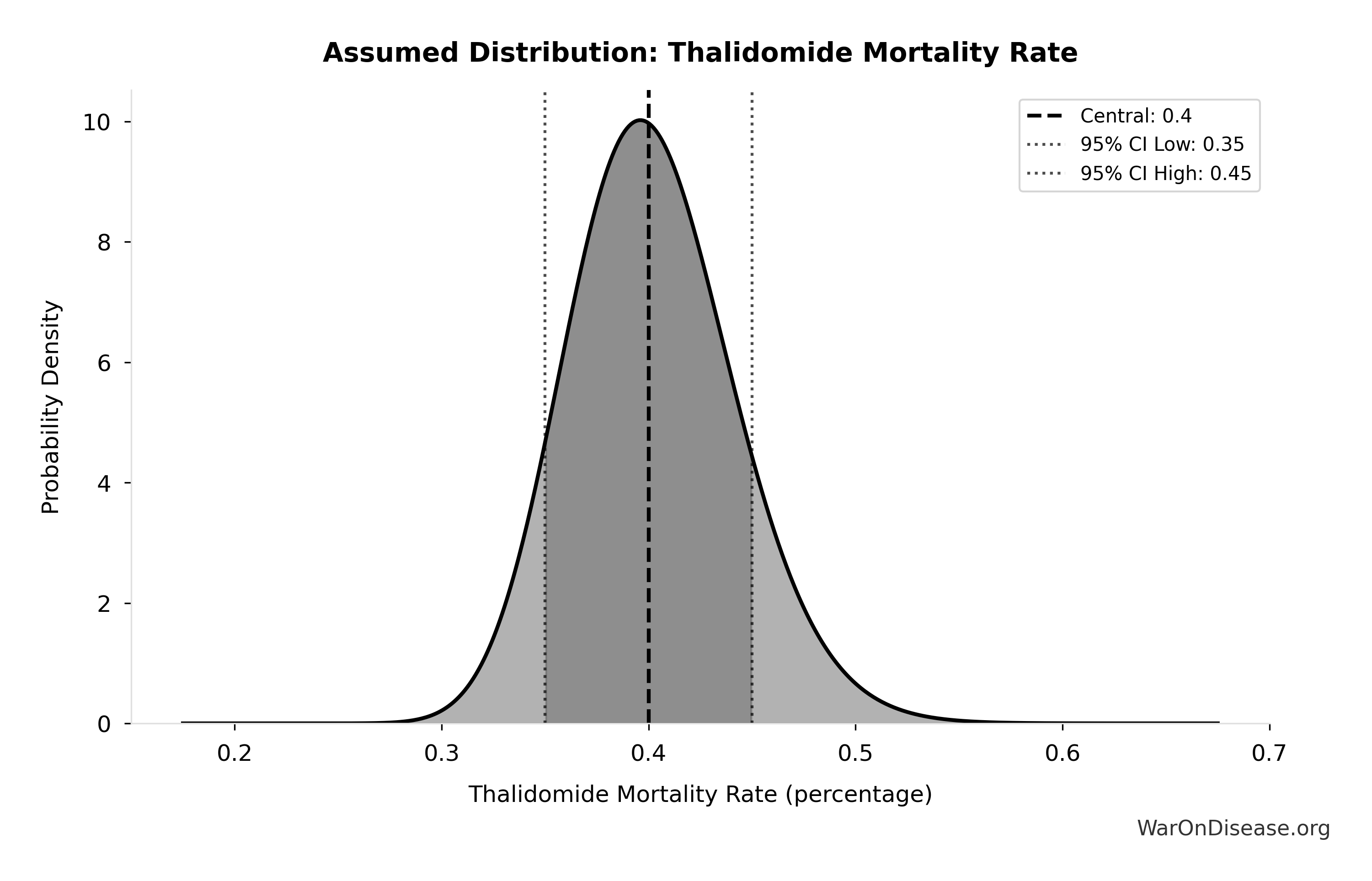
This chart shows the assumed probability distribution for this parameter. The shaded region represents the 95% confidence interval where we expect the true value to fall.
~ Medium confidence
Value of Statistical Life: $10M
Note📊 Details
Value of Statistical Life (conservative estimate)
Source:134
Uncertainty Range
Technical: 95% CI: [$5M, $15M] • Distribution: Gamma (SE: $3M)
What this means: There’s significant uncertainty here. The true value likely falls between $5M and $15M (±50%). This represents a wide range that our Monte Carlo simulations account for when calculating overall uncertainty in the results.
The gamma distribution means values follow a specific statistical pattern.
Input Distribution
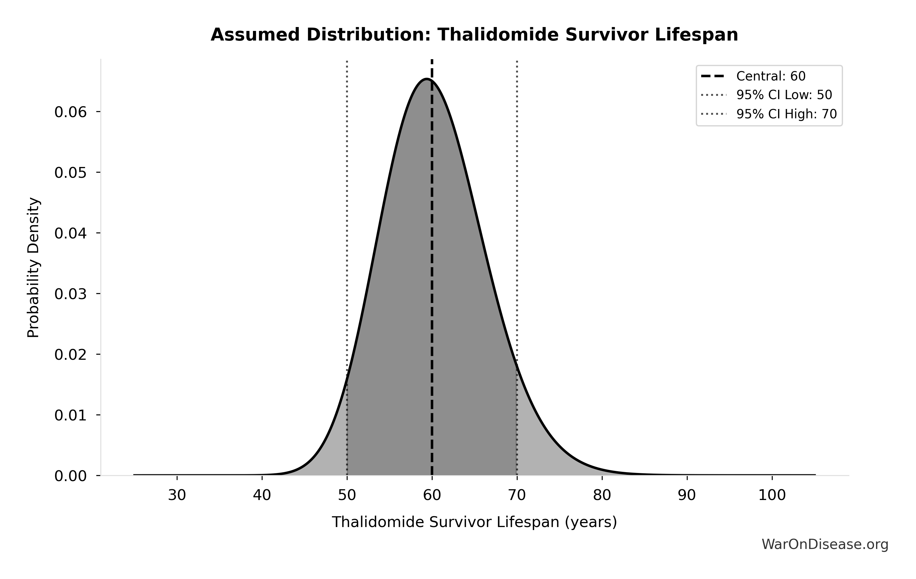
This chart shows the assumed probability distribution for this parameter. The shaded region represents the 95% confidence interval where we expect the true value to fall.
✓ High confidence
Vitamin A Supplementation Cost per DALY: $37
Note📊 Details
Cost per DALY for vitamin A supplementation programs (India: $23-50; Africa: $40-255; wide variation by region and baseline VAD prevalence). Using India midpoint as conservative estimate.
Source:135
~ Medium confidence
Return on Investment from Water Fluoridation Programs: 23:1
Note📊 Details
Cost-Effectiveness Threshold ($50,000/QALY): $50K
Note📊 Details
Cost-effectiveness threshold widely used in US health economics ($50,000/QALY, from 1980s dialysis costs)
Source:137
✓ High confidence
Core Definitions
Fundamental parameters and constants used throughout the analysis.
ADAPTABLE Trial Patients Enrolled: 15.1 thousand patients
Note📊 Details
Patients enrolled in ADAPTABLE trial (PCORnet 2016-2019). Enrolled across 40 clinical sites. Precise count from trial completion records.
Core definition
Percentage of Budget Defense Sector Keeps Under 1% treaty: 99%
Note📊 Details
Percentage of budget defense sector keeps under 1% treaty
Core definition
dFDA Annual Trial Funding: $21.8B
Note📊 Details
Assumed annual funding for dFDA pragmatic clinical trials (~$21.8B/year). Source-agnostic: could come from military reallocation, philanthropy, or government appropriation.
Uncertainty Range
Technical: Distribution: Fixed
Core definition
Years to Reach Full Decentralized Framework for Drug Assessment Adoption: 5 years
Note📊 Details
Years to reach full Decentralized Framework for Drug Assessment adoption
Core definition
Decentralized Framework for Drug Assessment Core framework Annual OPEX: $18.9M
Note📊 Details
Decentralized Framework for Drug Assessment Core framework annual opex (midpoint of $11-26.5M)
Uncertainty Range
Technical: 95% CI: [$11M, $26.5M] • Distribution: Lognormal
What this means: There’s significant uncertainty here. The true value likely falls between $11M and $26.5M (±41%). This represents a wide range that our Monte Carlo simulations account for when calculating overall uncertainty in the results.
The lognormal distribution means values can’t go negative and have a longer tail toward higher values (common for costs and populations).
Input Distribution
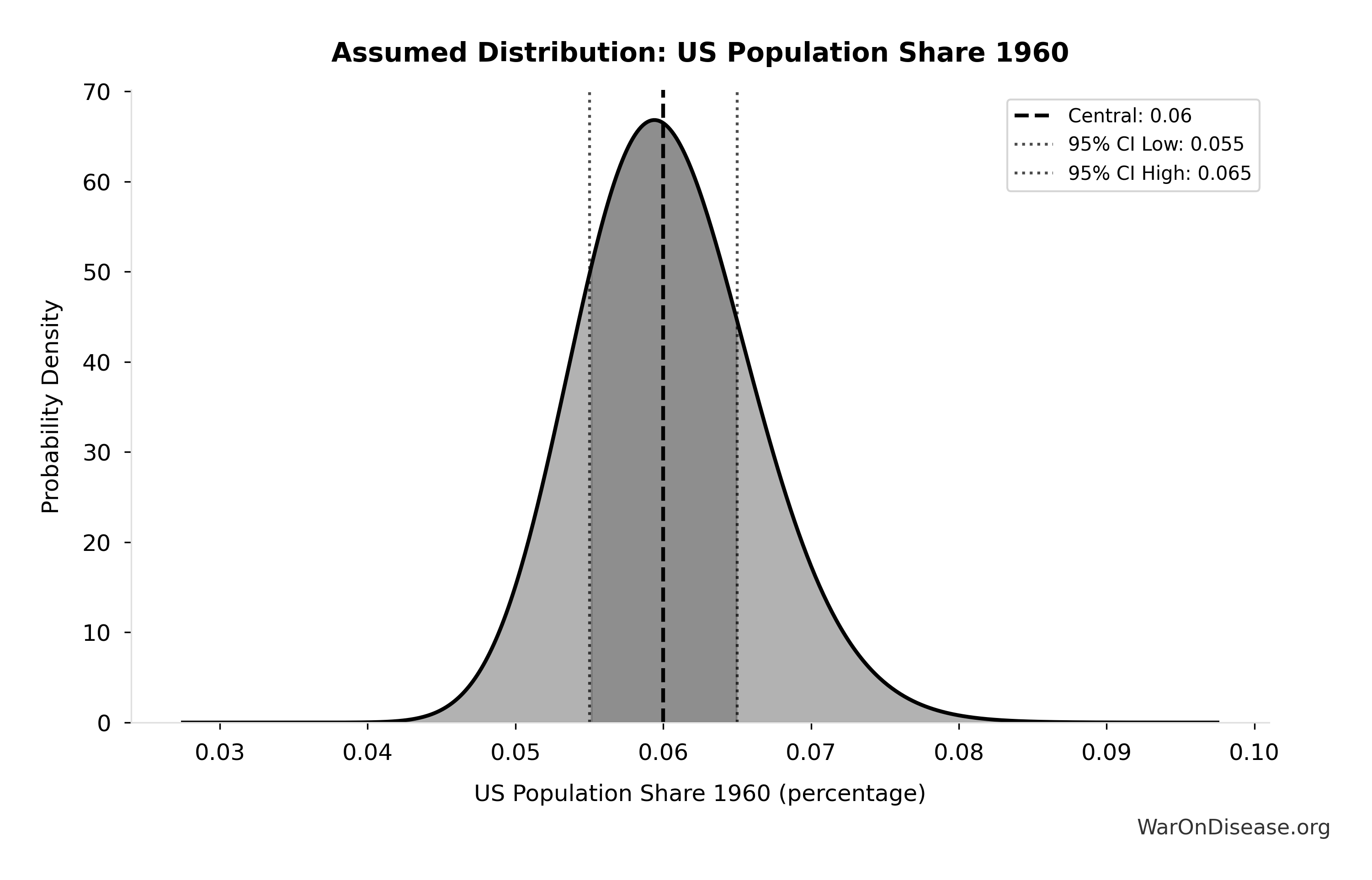
This chart shows the assumed probability distribution for this parameter. The shaded region represents the 95% confidence interval where we expect the true value to fall.
Core definition
Decentralized Framework for Drug Assessment Core framework Build Cost: $40M
Note📊 Details
Decentralized Framework for Drug Assessment Core framework build cost
Uncertainty Range
Technical: 95% CI: [$25M, $65M] • Distribution: Lognormal
What this means: There’s significant uncertainty here. The true value likely falls between $25M and $65M (±50%). This represents a wide range that our Monte Carlo simulations account for when calculating overall uncertainty in the results.
The lognormal distribution means values can’t go negative and have a longer tail toward higher values (common for costs and populations).
Input Distribution
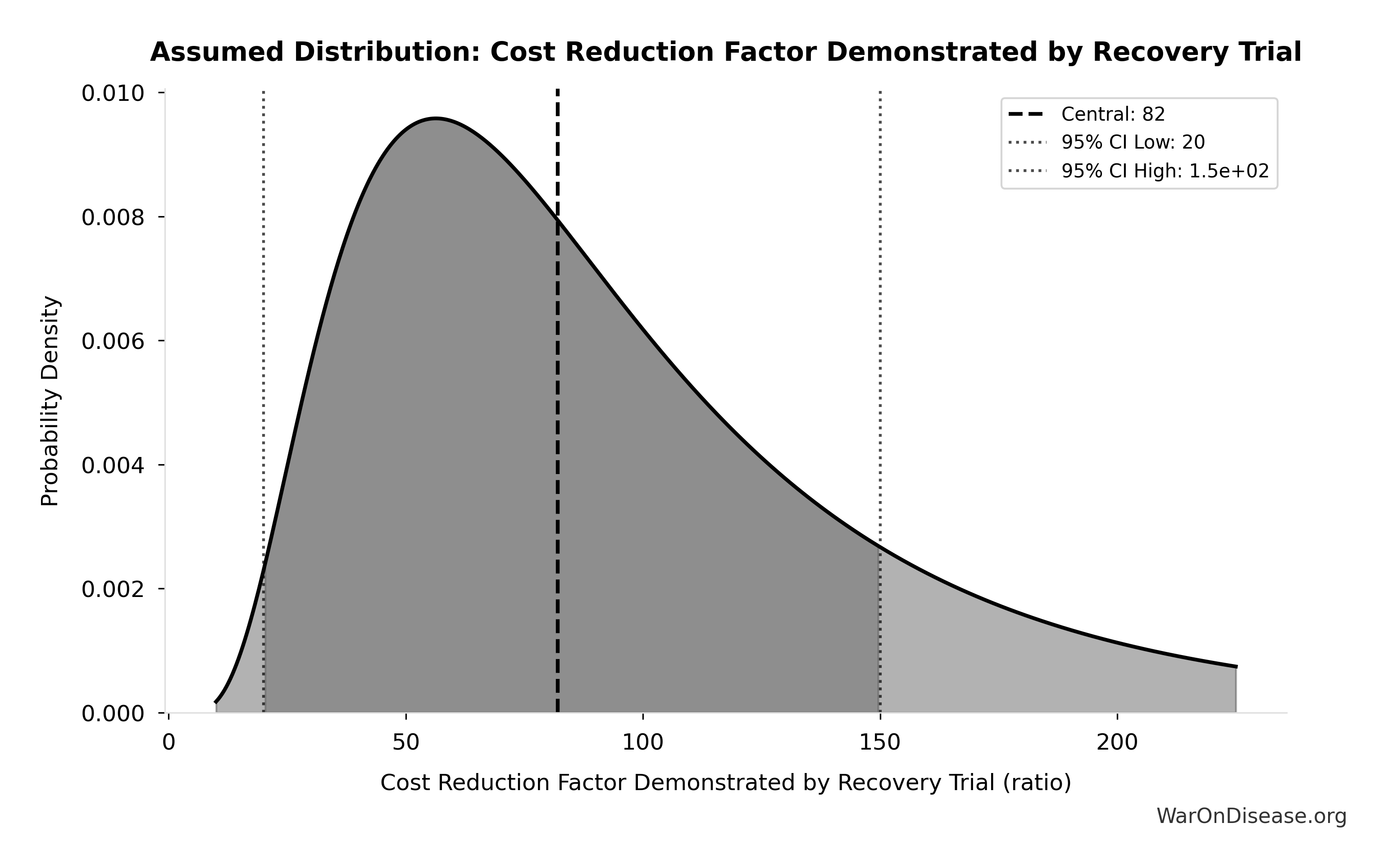
This chart shows the assumed probability distribution for this parameter. The shaded region represents the 95% confidence interval where we expect the true value to fall.
Core definition
Decentralized Framework for Drug Assessment Community Support Costs: $2M
Note📊 Details
Decentralized Framework for Drug Assessment community support costs
Uncertainty Range
Technical: 95% CI: [$1M, $3M] • Distribution: Lognormal
What this means: There’s significant uncertainty here. The true value likely falls between $1M and $3M (±50%). This represents a wide range that our Monte Carlo simulations account for when calculating overall uncertainty in the results.
The lognormal distribution means values can’t go negative and have a longer tail toward higher values (common for costs and populations).
Input Distribution
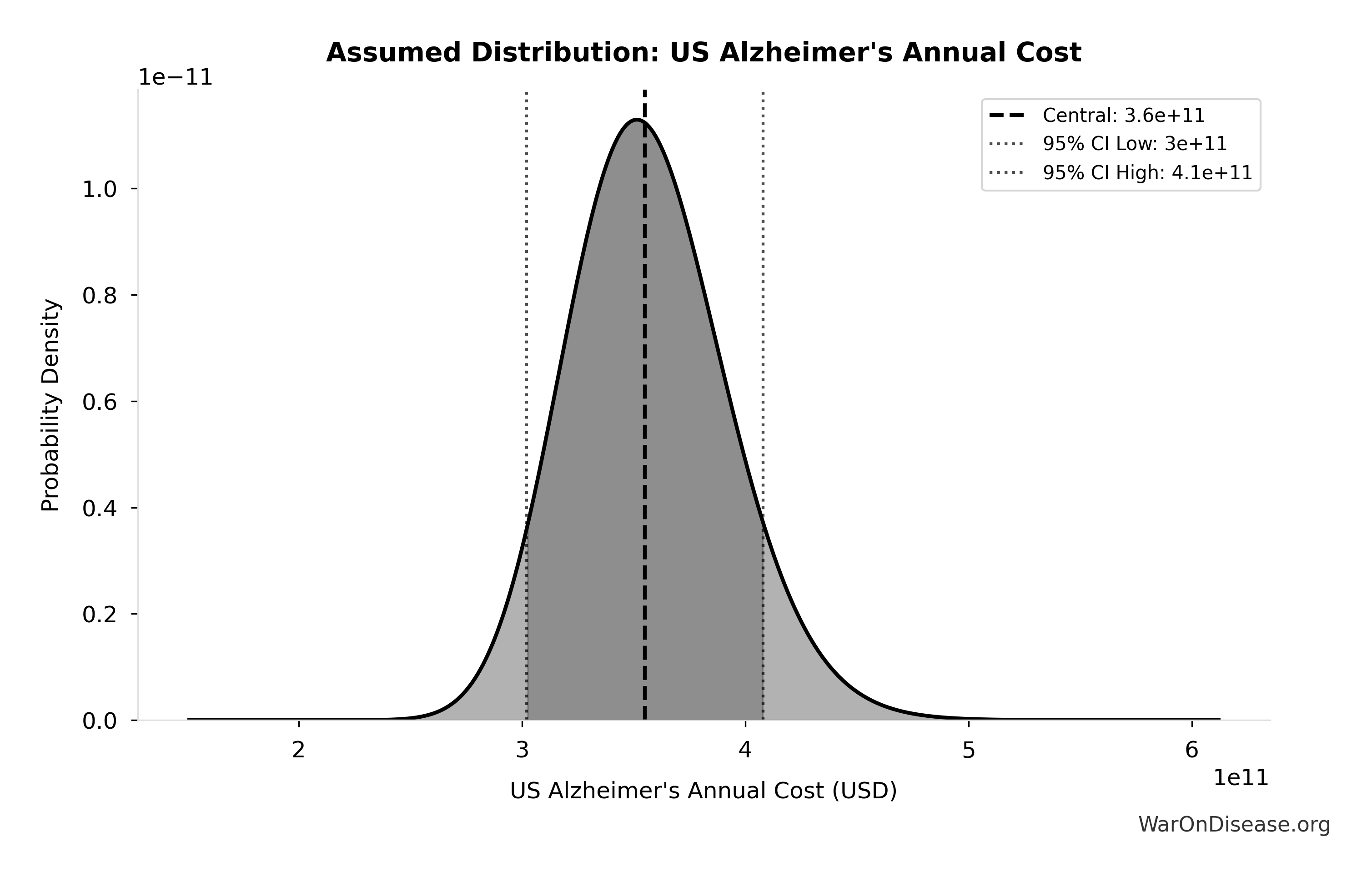
This chart shows the assumed probability distribution for this parameter. The shaded region represents the 95% confidence interval where we expect the true value to fall.
Core definition
Decentralized Framework for Drug Assessment Infrastructure Costs: $8M
Note📊 Details
Decentralized Framework for Drug Assessment infrastructure costs (cloud, security)
Uncertainty Range
Technical: 95% CI: [$5M, $12M] • Distribution: Lognormal
What this means: There’s significant uncertainty here. The true value likely falls between $5M and $12M (±44%). This represents a wide range that our Monte Carlo simulations account for when calculating overall uncertainty in the results.
The lognormal distribution means values can’t go negative and have a longer tail toward higher values (common for costs and populations).
Input Distribution
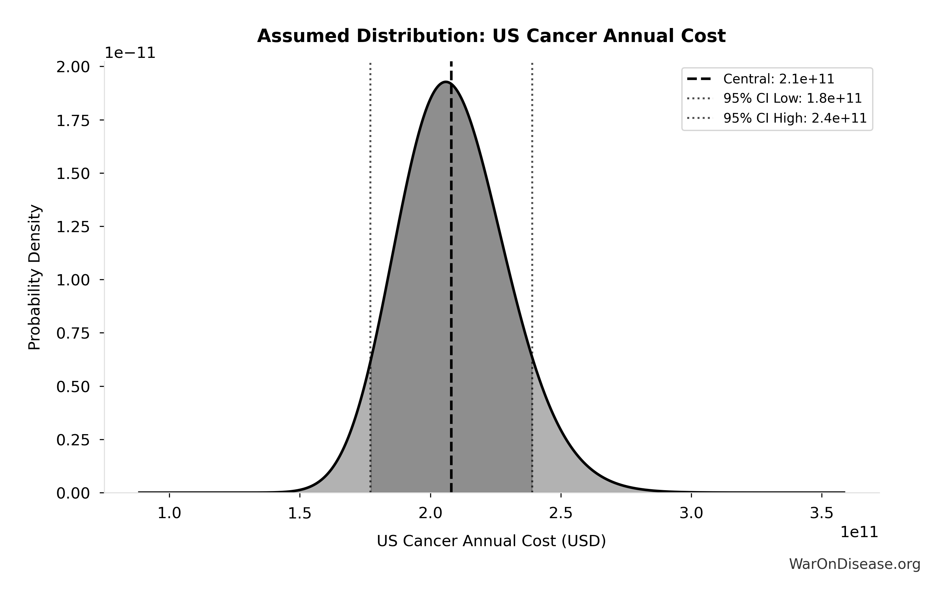
This chart shows the assumed probability distribution for this parameter. The shaded region represents the 95% confidence interval where we expect the true value to fall.
Core definition
Decentralized Framework for Drug Assessment Maintenance Costs: $15M
Note📊 Details
Decentralized Framework for Drug Assessment maintenance costs
Uncertainty Range
Technical: 95% CI: [$10M, $22M] • Distribution: Lognormal
What this means: There’s significant uncertainty here. The true value likely falls between $10M and $22M (±40%). This represents a wide range that our Monte Carlo simulations account for when calculating overall uncertainty in the results.
The lognormal distribution means values can’t go negative and have a longer tail toward higher values (common for costs and populations).
Input Distribution
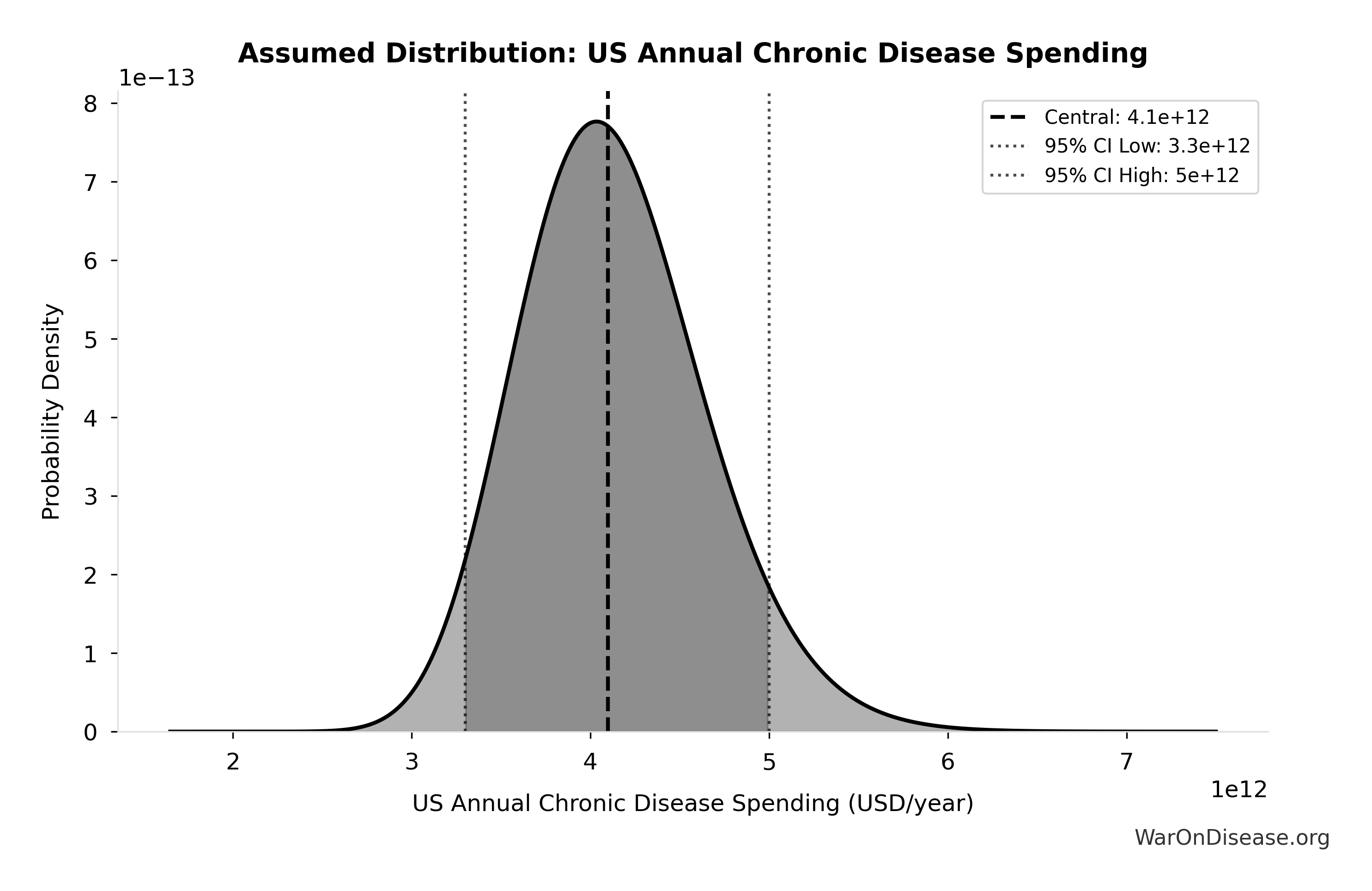
This chart shows the assumed probability distribution for this parameter. The shaded region represents the 95% confidence interval where we expect the true value to fall.
Core definition
Decentralized Framework for Drug Assessment Regulatory Coordination Costs: $5M
Note📊 Details
Decentralized Framework for Drug Assessment regulatory coordination costs
Uncertainty Range
Technical: 95% CI: [$3M, $8M] • Distribution: Lognormal
What this means: There’s significant uncertainty here. The true value likely falls between $3M and $8M (±50%). This represents a wide range that our Monte Carlo simulations account for when calculating overall uncertainty in the results.
The lognormal distribution means values can’t go negative and have a longer tail toward higher values (common for costs and populations).
Input Distribution
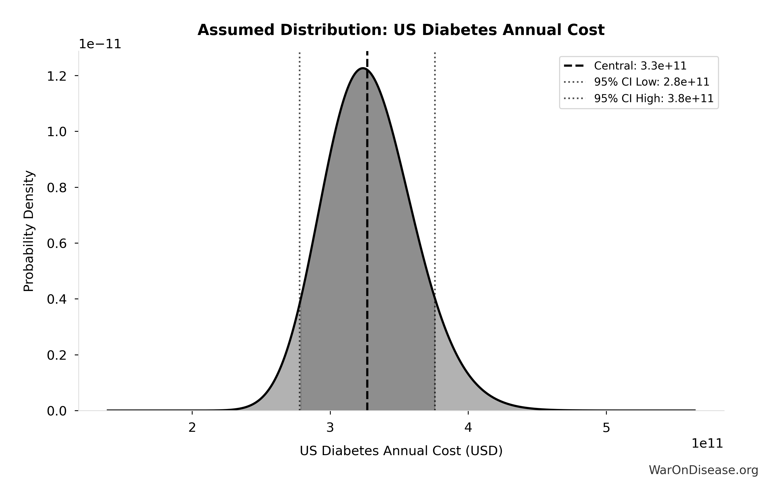
This chart shows the assumed probability distribution for this parameter. The shaded region represents the 95% confidence interval where we expect the true value to fall.
Core definition
Decentralized Framework for Drug Assessment Staff Costs: $10M
Note📊 Details
Decentralized Framework for Drug Assessment staff costs (minimal, AI-assisted)
Uncertainty Range
Technical: 95% CI: [$7M, $15M] • Distribution: Lognormal
What this means: There’s significant uncertainty here. The true value likely falls between $7M and $15M (±40%). This represents a wide range that our Monte Carlo simulations account for when calculating overall uncertainty in the results.
The lognormal distribution means values can’t go negative and have a longer tail toward higher values (common for costs and populations).
Input Distribution

This chart shows the assumed probability distribution for this parameter. The shaded region represents the 95% confidence interval where we expect the true value to fall.
Core definition
DIH Broader Initiatives Annual OPEX: $21.1M
Note📊 Details
DIH broader initiatives annual opex (medium case)
Uncertainty Range
Technical: 95% CI: [$14M, $32M] • Distribution: Lognormal
What this means: There’s significant uncertainty here. The true value likely falls between $14M and $32M (±43%). This represents a wide range that our Monte Carlo simulations account for when calculating overall uncertainty in the results.
The lognormal distribution means values can’t go negative and have a longer tail toward higher values (common for costs and populations).
Input Distribution
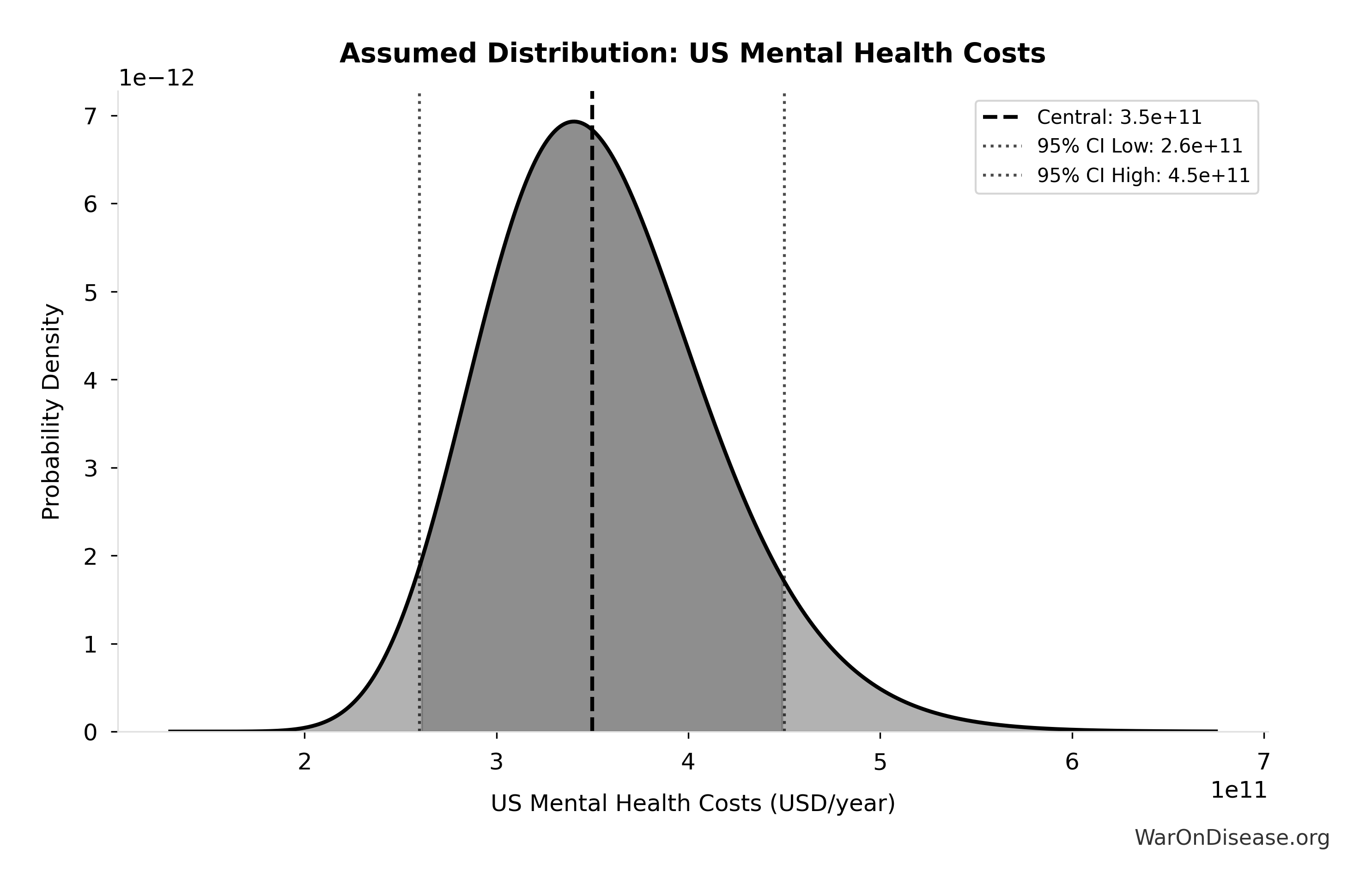
This chart shows the assumed probability distribution for this parameter. The shaded region represents the 95% confidence interval where we expect the true value to fall.
Core definition
DIH Broader Initiatives Upfront Cost: $230M
Note📊 Details
DIH broader initiatives upfront cost (medium case)
Uncertainty Range
Technical: 95% CI: [$150M, $350M] • Distribution: Lognormal
What this means: There’s significant uncertainty here. The true value likely falls between $150M and $350M (±44%). This represents a wide range that our Monte Carlo simulations account for when calculating overall uncertainty in the results.
The lognormal distribution means values can’t go negative and have a longer tail toward higher values (common for costs and populations).
Input Distribution
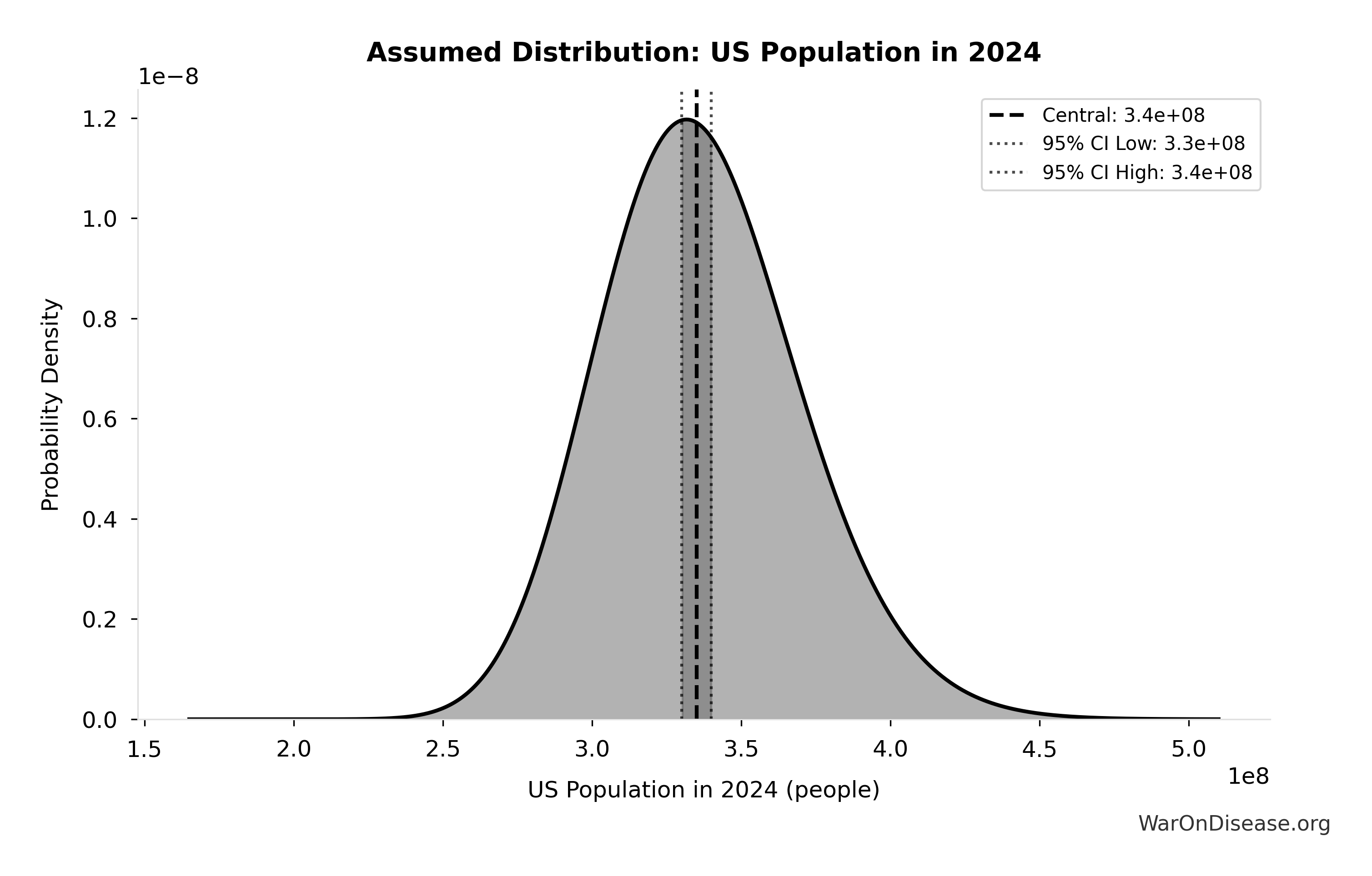
This chart shows the assumed probability distribution for this parameter. The shaded region represents the 95% confidence interval where we expect the true value to fall.
Core definition
Eventually Avoidable DALY Percentage: 92.6%
Note📊 Details
Percentage of DALYs that are eventually avoidable with sufficient biomedical research. Uses same methodology as EVENTUALLY_AVOIDABLE_DEATH_PCT. Most non-fatal chronic conditions (arthritis, depression, chronic pain) are also addressable through research, so the percentage is similar to deaths.
Uncertainty Range
Technical: 95% CI: [50%, 98%] • Distribution: Beta
What this means: There’s significant uncertainty here. The true value likely falls between 50% and 98% (±26%). This represents a wide range that our Monte Carlo simulations account for when calculating overall uncertainty in the results.
The beta distribution means values are bounded and can skew toward one end.
Input Distribution
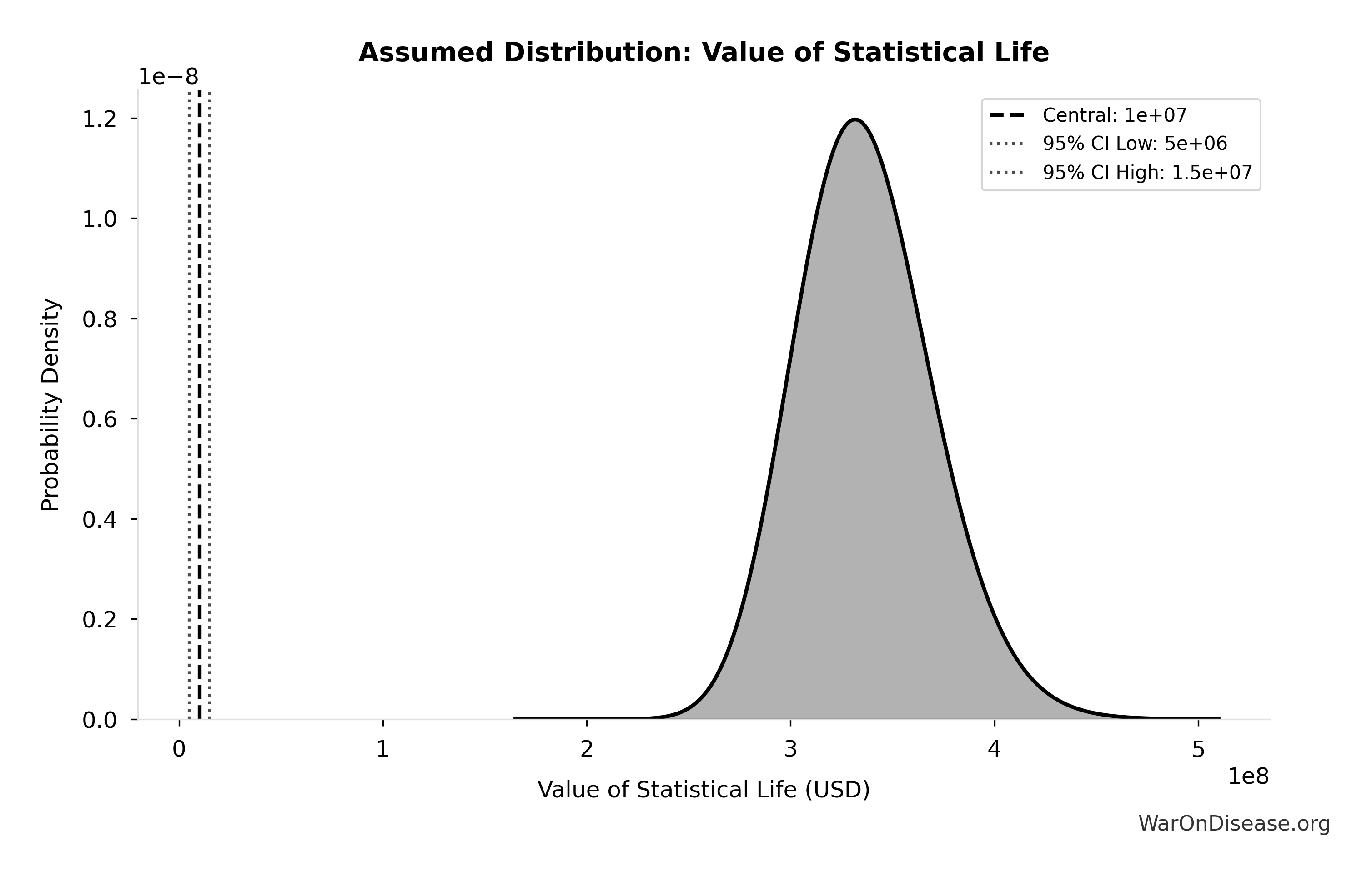
This chart shows the assumed probability distribution for this parameter. The shaded region represents the 95% confidence interval where we expect the true value to fall.
Core definition
Eventually Avoidable Death Percentage: 92.6%
Note📊 Details
Percentage of deaths that are eventually avoidable with sufficient biomedical research and technological advancement. Central estimate ~92% based on ~7.9% fundamentally unavoidable (primarily accidents). Wide uncertainty reflects debate over: (1) aging as addressable vs. fundamental, (2) asymptotic difficulty of last diseases, (3) multifactorial disease complexity.
Uncertainty Range
Technical: 95% CI: [50%, 98%] • Distribution: Beta
What this means: There’s significant uncertainty here. The true value likely falls between 50% and 98% (±26%). This represents a wide range that our Monte Carlo simulations account for when calculating overall uncertainty in the results.
The beta distribution means values are bounded and can skew toward one end.
Input Distribution
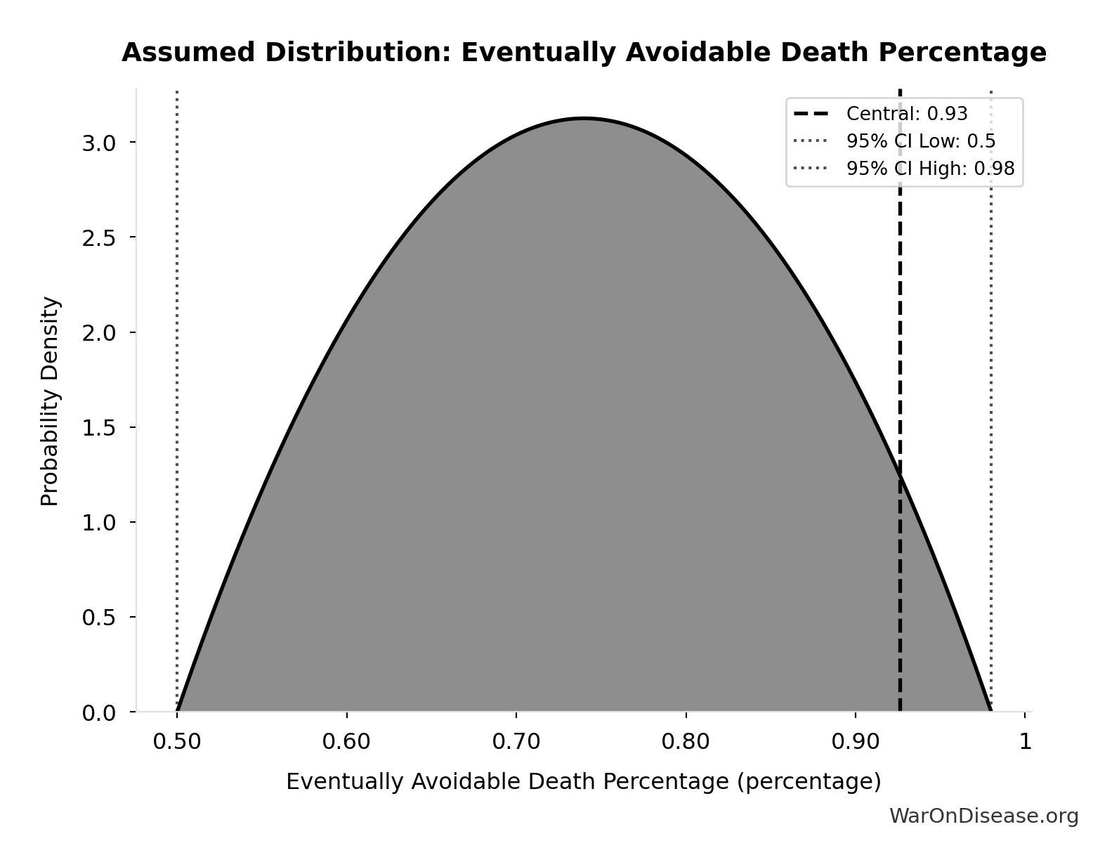
This chart shows the assumed probability distribution for this parameter. The shaded region represents the 95% confidence interval where we expect the true value to fall.
Core definition
Baseline Global GDP Growth Rate: 2.5%
Note📊 Details
Status-quo baseline annual global GDP growth rate.
Uncertainty Range
Technical: Distribution: Fixed
Core definition
IAB Political Incentive Funding Percentage: 10%
Note📊 Details
Percentage of treaty funding allocated to Incentive Alignment Bond mechanism for political incentives (independent expenditures/PACs, post-office fellowships, Public Good Score infrastructure)
Uncertainty Range
Technical: Distribution: Fixed
Core definition
GDP Growth Boost at 30% Military Reallocation: 5.5%
Note📊 Details
Historical calibration target: 30% military reallocation maps to ~5.5 percentage points annual GDP growth boost.
Uncertainty Range
Technical: 95% CI: [3.5%, 7.5%] • Distribution: Normal (SE: 1%)
What this means: There’s significant uncertainty here. The true value likely falls between 3.5% and 7.5% (±36%). This represents a wide range that our Monte Carlo simulations account for when calculating overall uncertainty in the results.
The normal distribution means values cluster around the center with equal chances of being higher or lower.
Input Distribution
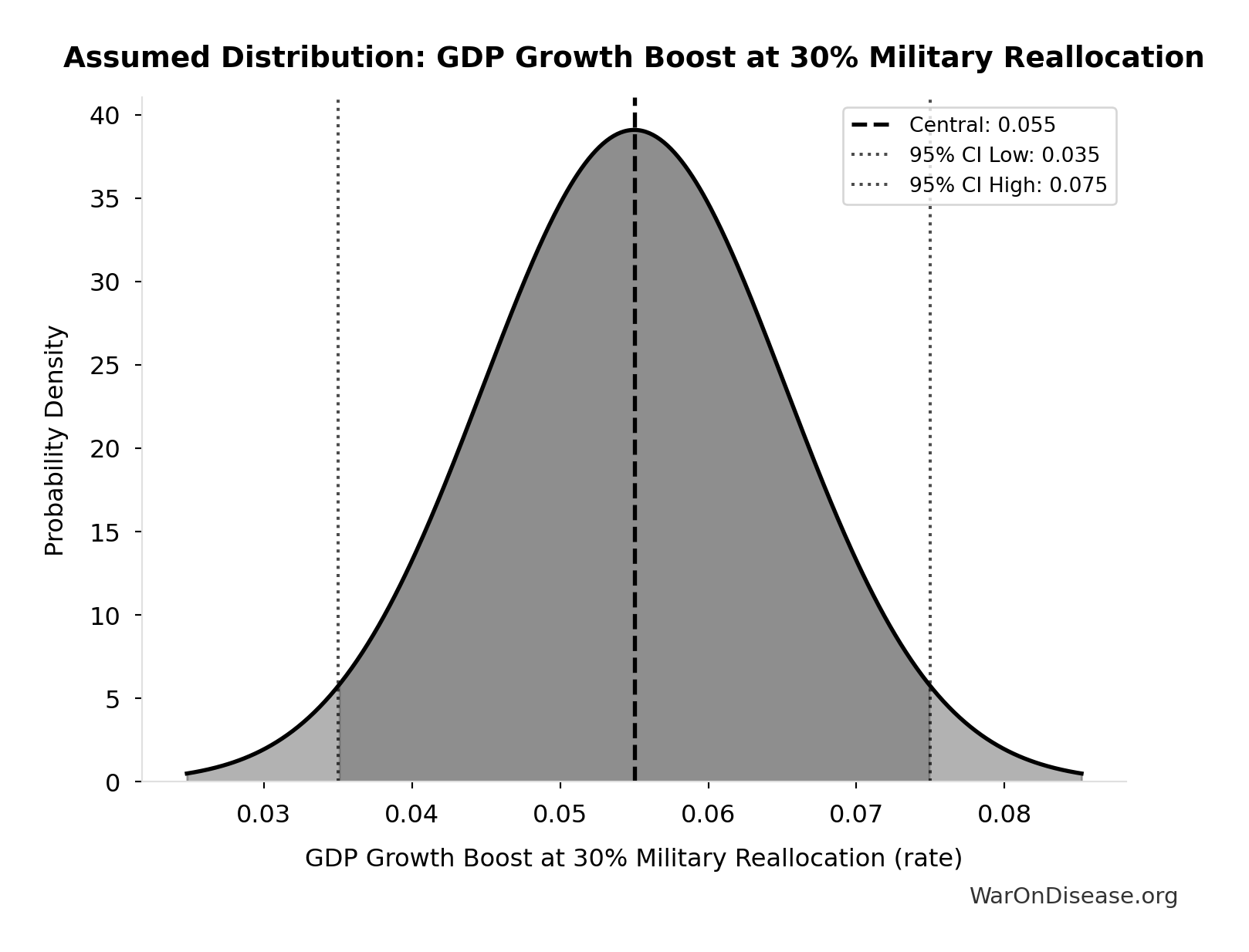
This chart shows the assumed probability distribution for this parameter. The shaded region represents the 95% confidence interval where we expect the true value to fall.
Core definition
Standard Discount Rate for NPV Analysis: 3%
Note📊 Details
Standard discount rate for NPV analysis (3% annual, social discount rate)
Uncertainty Range
Technical: Distribution: Fixed
Core definition
Standard Time Horizon for NPV Analysis: 10 years
Note📊 Details
Standard time horizon for NPV analysis
Uncertainty Range
Technical: Distribution: Fixed
Core definition
Direct Fiscal Savings from 1% Military Spending Reduction: $27.2B
Note📊 Details
Direct fiscal savings from 1% military spending reduction (high confidence)
Core definition
Pre-1962 Validation Years: 77 years
Note📊 Details
Years of empirical validation for physician-led pragmatic trials (1883-1960)
Core definition
QALYs per COVID Death Averted: 5 QALYs/death
Note📊 Details
Average QALYs gained per COVID death averted. Conservative estimate reflecting older age distribution of COVID mortality. See confidence_interval for range.
Uncertainty Range
Technical: 95% CI: [3 QALYs/death, 10 QALYs/death] • Distribution: Lognormal
What this means: This estimate is highly uncertain. The true value likely falls between 3 QALYs/death and 10 QALYs/death (±70%). This represents a very wide range that our Monte Carlo simulations account for when calculating overall uncertainty in the results.
The lognormal distribution means values can’t go negative and have a longer tail toward higher values (common for costs and populations).
Input Distribution
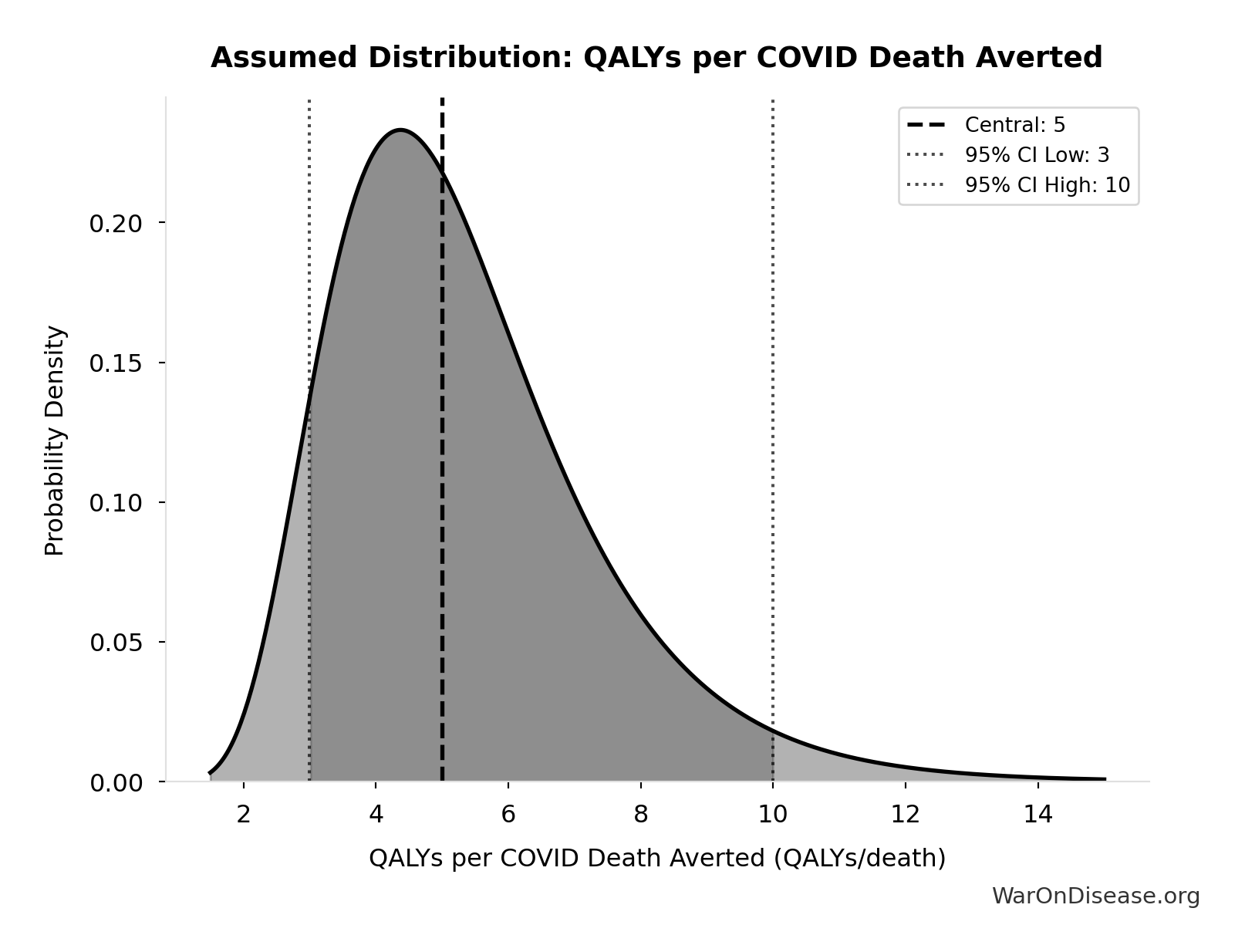
This chart shows the assumed probability distribution for this parameter. The shaded region represents the 95% confidence interval where we expect the true value to fall.
Core definition
R&D Spillover Multiplier: 2x
Note📊 Details
R&D spillover multiplier: each $1 in directed medical research produces $2 in adjacent sector GDP growth (biotech, AI, computing, materials science, manufacturing). Conservative estimate; military R&D spillover produced the internet, GPS, jet engines. Medical R&D spillover already produced CRISPR, mRNA platforms, AI protein folding.
Uncertainty Range
Technical: 95% CI: [1.5x, 2.5x] • Distribution: Normal (SE: 0.25x)
What this means: This estimate has moderate uncertainty. The true value likely falls between 1.5x and 2.5x (±25%). This represents a reasonable range that our Monte Carlo simulations account for when calculating overall uncertainty in the results.
The normal distribution means values cluster around the center with equal chances of being higher or lower.
Input Distribution
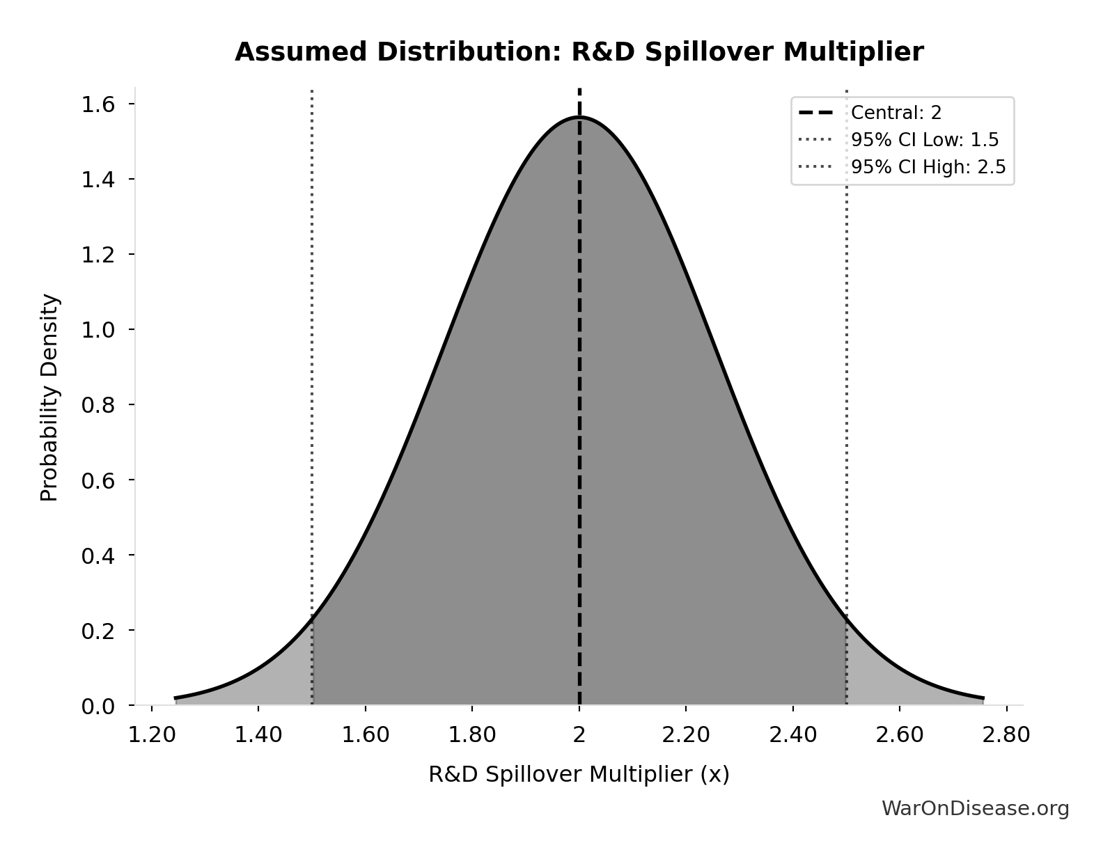
This chart shows the assumed probability distribution for this parameter. The shaded region represents the 95% confidence interval where we expect the true value to fall.
Core definition
Safe Compounds Available for Testing: 9.5 thousand compounds
Note📊 Details
Total safe compounds available for repurposing (FDA-approved + GRAS substances, midpoint of 7,000-12,000 range)
Uncertainty Range
Technical: 95% CI: [7 thousand compounds, 12 thousand compounds] • Distribution: Uniform
What this means: There’s significant uncertainty here. The true value likely falls between 7 thousand compounds and 12 thousand compounds (±26%). This represents a wide range that our Monte Carlo simulations account for when calculating overall uncertainty in the results.
The uniform distribution means any value in the range is equally likely.
Input Distribution
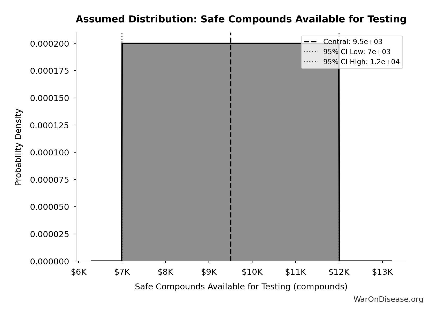
This chart shows the assumed probability distribution for this parameter. The shaded region represents the 95% confidence interval where we expect the true value to fall.
Core definition
Tested Drug-Disease Relationships: 32.5 thousand relationships
Note📊 Details
Estimated drug-disease relationships actually tested (approved uses + repurposed + failed trials, midpoint of 15,000-50,000 range)
Uncertainty Range
Technical: 95% CI: [15 thousand relationships, 50 thousand relationships] • Distribution: Lognormal
What this means: This estimate is highly uncertain. The true value likely falls between 15 thousand relationships and 50 thousand relationships (±54%). This represents a very wide range that our Monte Carlo simulations account for when calculating overall uncertainty in the results.
The lognormal distribution means values can’t go negative and have a longer tail toward higher values (common for costs and populations).
Input Distribution
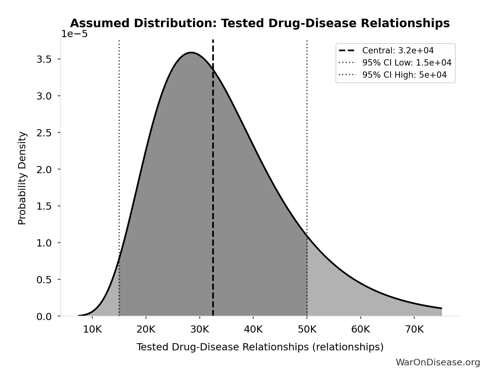
This chart shows the assumed probability distribution for this parameter. The shaded region represents the 95% confidence interval where we expect the true value to fall.
Core definition
Political Lobbying Campaign: Direct Lobbying, Super Pacs, Opposition Research, Staff, Legal/Compliance: $650M
Note📊 Details
Political lobbying campaign: direct lobbying (US/EU/G20), Super PACs, opposition research, staff, legal/compliance. Budget exceeds combined pharma ($300M/year) and military-industrial complex ($150M/year) lobbying to ensure competitive positioning. Referendum relies on grassroots mobilization and earned media, while lobbying requires matching or exceeding opposition spending for political viability.
Uncertainty Range
Technical: 95% CI: [$325M, $1.3B] • Distribution: Lognormal
What this means: This estimate is highly uncertain. The true value likely falls between $325M and $1.3B (±75%). This represents a very wide range that our Monte Carlo simulations account for when calculating overall uncertainty in the results.
The lognormal distribution means values can’t go negative and have a longer tail toward higher values (common for costs and populations).
Input Distribution
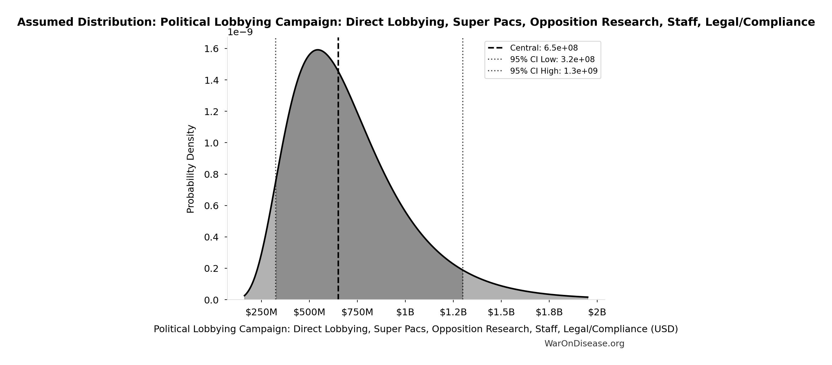
This chart shows the assumed probability distribution for this parameter. The shaded region represents the 95% confidence interval where we expect the true value to fall.
Core definition
Reserve Fund / Contingency Buffer: $100M
Note📊 Details
Reserve fund / contingency buffer (10% of total campaign cost). Using industry standard 10% for complex campaigns with potential for unforeseen legal challenges, opposition response, or regulatory delays. Conservative lower bound of $20M (2%) reflects transparent budget allocation and predictable referendum/lobbying costs.
Uncertainty Range
Technical: 95% CI: [$20M, $150M] • Distribution: Lognormal
What this means: This estimate is highly uncertain. The true value likely falls between $20M and $150M (±65%). This represents a very wide range that our Monte Carlo simulations account for when calculating overall uncertainty in the results.
The lognormal distribution means values can’t go negative and have a longer tail toward higher values (common for costs and populations).
Input Distribution
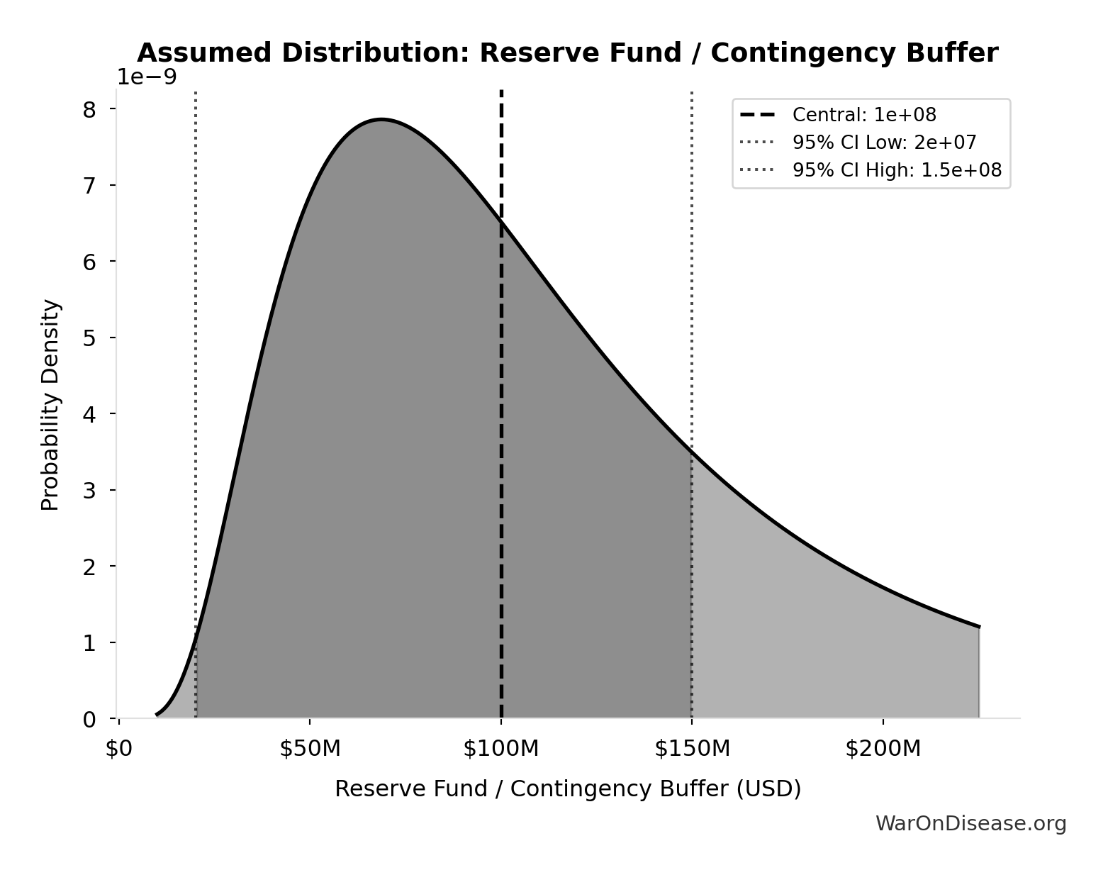
This chart shows the assumed probability distribution for this parameter. The shaded region represents the 95% confidence interval where we expect the true value to fall.
Core definition
Viral Referendum Budget: $250M
Note📊 Details
Viral referendum budget for 280M verified votes (base: $250M realistic with $0.50/vote avg, range: $150M optimistic $0.20/vote to $410M worst-case $1.05/vote). Components: platform ($35M), verification infrastructure (280M × friction × $0.18-0.20), tiered referral payments (varies by virality and marginal cost curve per diffusion theory), marketing seed ($5-15M). Based on PayPal referral economics ($18-36 inflation-adjusted) and biometric verification pricing ($0.15-0.25 at 300M+ scale).
Uncertainty Range
Technical: 95% CI: [$150M, $410M]
What this means: This estimate is highly uncertain. The true value likely falls between $150M and $410M (±52%). This represents a very wide range that our Monte Carlo simulations account for when calculating overall uncertainty in the results.
Input Distribution
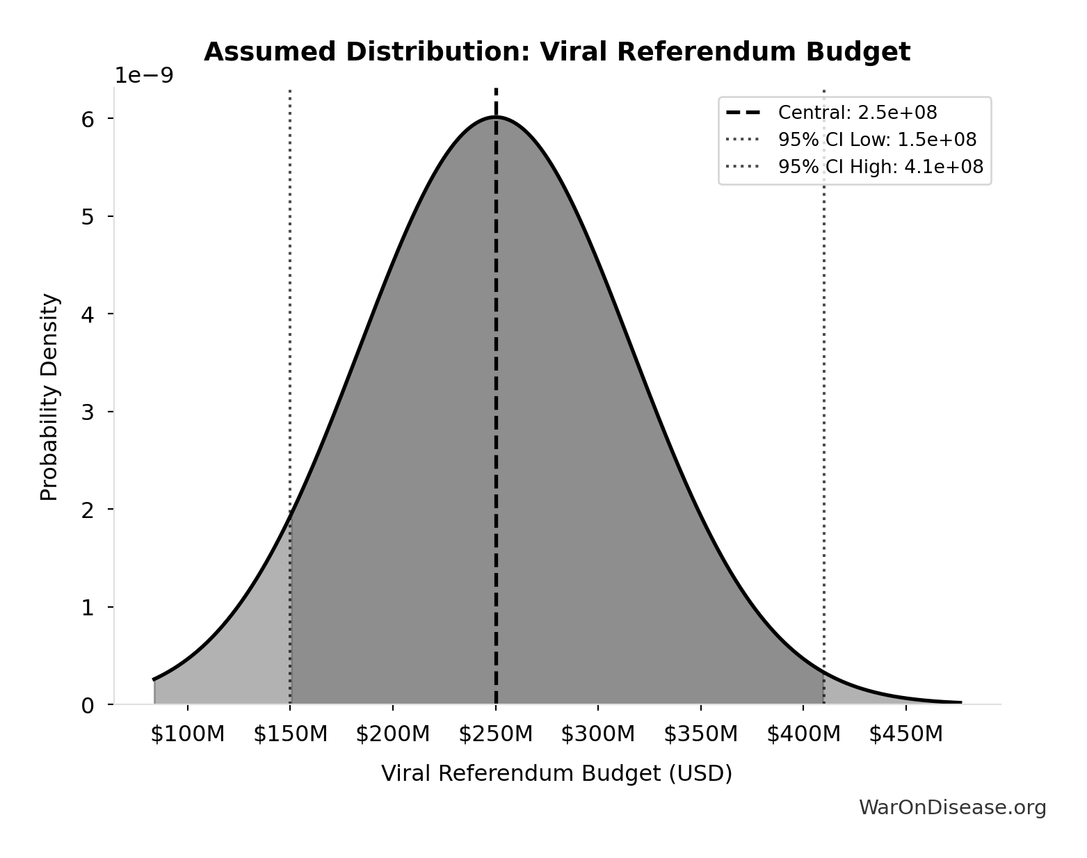
This chart shows the assumed probability distribution for this parameter. The shaded region represents the 95% confidence interval where we expect the true value to fall.
Core definition
1% Reduction in Military Spending/War Costs from Treaty: 1%
Note📊 Details
1% reduction in military spending/war costs from treaty
Uncertainty Range
Technical: Distribution: Fixed
Core definition
Trial-Relevant Diseases: 1 thousand diseases
Note📊 Details
Consolidated count of trial-relevant diseases worth targeting (after grouping ICD-10 codes)
Uncertainty Range
Technical: 95% CI: [800 diseases, 1.2 thousand diseases] • Distribution: Uniform
What this means: This estimate has moderate uncertainty. The true value likely falls between 800 diseases and 1.2 thousand diseases (±20%). This represents a reasonable range that our Monte Carlo simulations account for when calculating overall uncertainty in the results.
The uniform distribution means any value in the range is equally likely.
Input Distribution
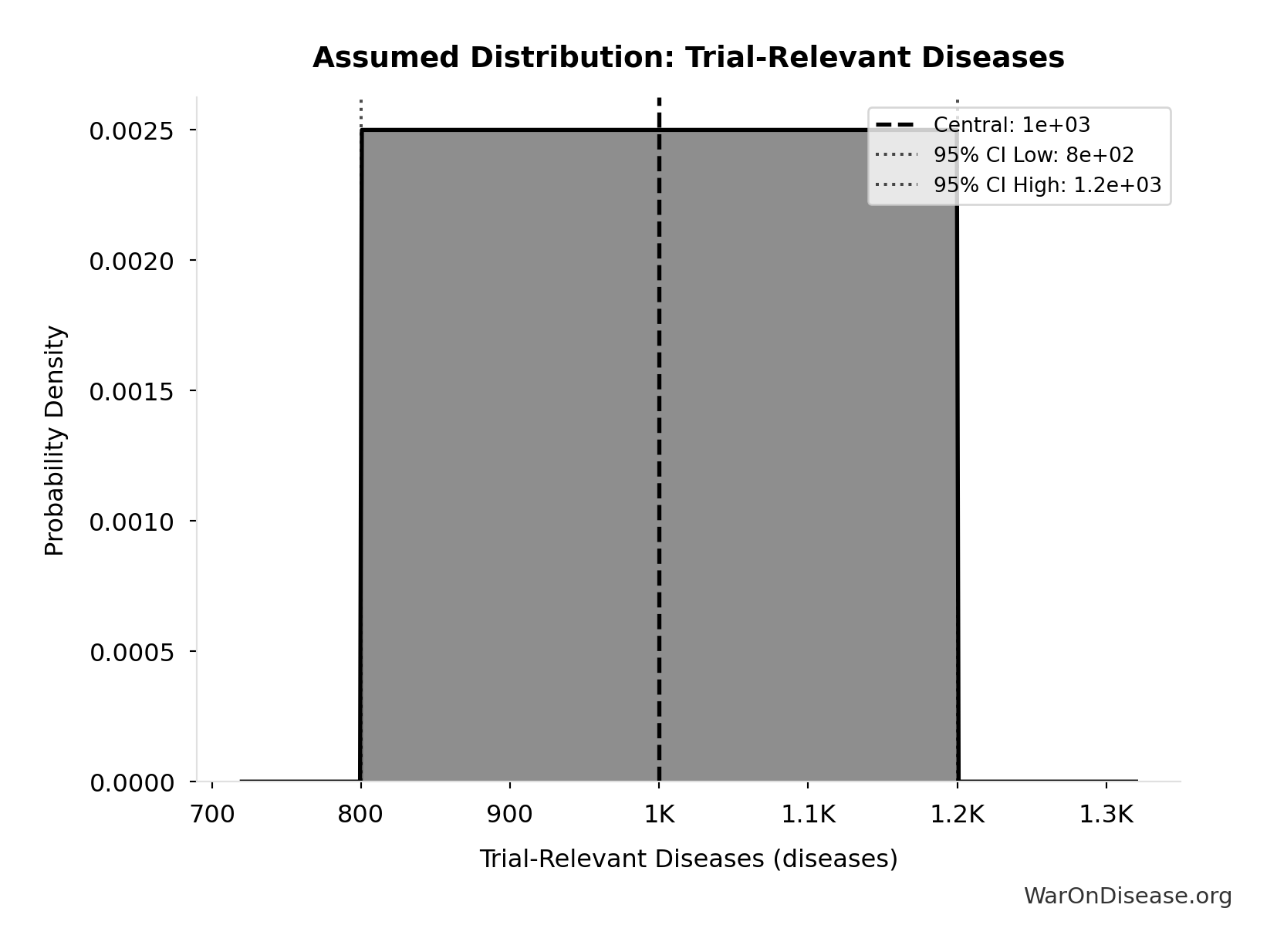
This chart shows the assumed probability distribution for this parameter. The shaded region represents the 95% confidence interval where we expect the true value to fall.
Core definition
Percentage of Captured Dividend Funding VICTORY Incentive Alignment Bonds: 10%
Note📊 Details
Percentage of captured dividend funding VICTORY Incentive Alignment Bonds (10%)
Uncertainty Range
Technical: Distribution: Fixed
Core definition